I hate IDL

I've been working a little bit in IDL for this new project because all the data is in fits files, Alexie has a lot of code that is in IDL which we are using to handle the CFHT data.

Anyway, I spent all morning struggling trying to do very simple input and output from this stupid stupid language.

I learned a few things, and since I hardly ever code in IDL, I am sure I'll forget unless I write them down right now. So here we go:

1) Tag names

You can get the tag names from a structure like this:

tname = tag_names(struct)

2) Merging structures

You can merge two structures as follows:

str3 = create_struct(str1,str2,NAME='str3')

3) writecol bug

For some reason when I try to use writecol to write out data, if there are more that 6 columns, and I don't specify the format, it puts a return carriage in the middle of the data. This goes away if you specify the format:

thisfile = './qsosMergedInfo.dat'
writecol,thisfile, qsos.ra, qsos.dec, qsos.z, qsos.zwarning, $
qsos.flux_clip_mean[0],qsos.flux_clip_mean[1], qsos.flux_clip_mean[2], $
qsos.flux_clip_mean[3], qsos.flux_clip_mean[4], fmt='(f,f,f,f,f,f,f,f,f)'

Reconstruction for Alexia

I'm back in Berkeley and very grateful to be in the cool weather and sleeping in my own bed. I seriously don't know how East Coast people handle that summer humidity.

I've spent the day getting my reconstruction code into shape for passing it over to Alexia to debug. Some lessons learned today are as follows:

1) I need to stop doing this "copy and paste" thing with python. Time to write up some more functions and get everything in execution mode... Alexia is right, I am wrong.

2) Some plotting tricks:
I've turned my plotting code into some plotting functions (see plotWPS and plotXi functions ../pythonjess/correlationData.py).

These functions now save the plots into the runDirectory as png files. You can look at them over terminal by typing:

> display plotname.png

They look like this (well why are white on black,
I need to figure out how to make them be white-on-black)

If you look at the inner working of these functions I use some commands do the pylab.gcf to set the size and print to a file. I think somewhere in there I can set up a color scheme. Should look into this. I used this web page to help me configure the above plot though.

3) I still don't really understand the different types of ways to write python functions. I've been defining functions as follows:

def function(arguments):
.
.
----Insert function code here
.
.
----return(thing to return)

However it seems like I can also just have a set of code (like a main function in C) that calls a bunch of other functions and isn't a self-contained function... and Demitri said that I just need the following line at the top of the code to make it executable in python:
#!/usr/bin/python

But then at scicoder, Demitri also said that I should create everything as a class. So I guess I just need to figure out what the difference between a class, def, and then just code in a file is.... Maybe Demitri, Alexia, Josh or Adam can help me?

However, as a result of all this effort, I now have code that runs the reconstruction from head-to-tail, and re-runs it once you have already made the correlation functions, and re-runs it with different phi-binning. They are in the following files:

../pythonjess/jessreconstructionFull.py
../pythonjess/jessreconstruction.py
../pythonjess/rerunjessreconstruction.py

These files are the logfiles for today.

Best reconstruction Plot:

=

Coding Wisdom from David Hogg

David Hogg came Scicoder to talk to us about Test-Driven Coding. He is pretty awesome.

Testing Your Code
1 bug / 1000 lines of code.

Ways to deal with this:
1) Test Driving Programming
2) Open-Source
3) Do Science with Code

Extreme Coding
1) Pair coding (coding together)
2) Stand up meetings (don't talk -- do)
3) Test Driving Programming (see below)
4) Minimal Implementation (re-factor frequently) only code things that you are actually going to use.

Test-Driven Programming

1) First write a test function to perform all possible tests you can imagine for your function.
2) Then run write the function and see how many of the tests it passes...
3) Keep modifying your function until it passes all the tests
4) Can't use code, check into repository unless it passes all tests

Functional Testing
1) Generate fake data + garbage
2) Run code
3) Did you get back what you put in?
4) Put assert statements in your code, such that if these assertions fail your code fails and spits out an error.

Have to be careful not to generate fake data that covered the entire spectrum of properties of your real data --- thus you could not be testing all cases or making all possible assertions.


But at the end of the day... what we really care about it this:
How do I know that my results are correct? ← (Probably not answerable)
or in real life...
Why do I think that my students results are correct?
- You do science with real data.
- You get results that you think you can publish and people will believe you (seriously this is what he said).

Blanton et. al. Luminosity Function Paper was originally a test by Mike Blanton to see if the SDSS data software pipeline was working and turned into one of the highest refereed papers out of the Sloan Survey. Thus testing really does matter.

On a side note, a link to my blog made it into Hogg's blog, and the thus circle is now complete.

Useful IDL Commands

I need to do some work for the likelihood project and thus code in IDL again. Because I am not working in IDL very frequently, I tend to forgot commands and syntax. I thought it would be useful to compile a list of commands here so that I don't have to keep looking these up again and again.

number of elements in an array:
print, N_ELEMENTS(array)

unix command in idl: dollar sign ($) before command
$pwd
$ls

list all variables currently being used:
help

doc_library, 'spherematch' -- man page for the function

which, 'spherematch' --- tells you where in the IDL path the function is.

when recompiling idlutils need to use evilmake

!pi is constant pi

plothist (makes histogram plot)

when looking at a structure you use the /str command:
help, mystructure, /str

reading a fits file using mrdfits:
filedata = mrdfits(file2read, 1)

Combine two structures of the same size:
struct3 =struct_combine(struct1,struct2)
Concatenate two structure of the same type:
struct3 = [struct1, struct2]

Plotting Histogram (from here):

PRO t_histogram
data = [[-5,  4,   2,  -8,  1], $
[ 3,  0,   5,  -5,  1], $
[ 6, -7,   4,  -4, -8], $
[-1, -5, -14,   2,  1]]
hist = HISTOGRAM(data)
bins = FINDGEN(N_ELEMENTS(hist)) + MIN(data)
PRINT, MIN(hist)
PRINT, bins
SPLOT, bins, hist, YRANGE = [MIN(hist)-1, MAX(hist)+1], PSYM = 10, XTITLE = 'Bin Number', YTITLE = 'Density per Bin'
END 

If you add maxmatch=1 to your spherematch it will avoid duplicates (should default to this)


total with higher precision: total(...., /double)


in for loops:
for j = 0L, rsize-1 do begin

the L makes j a long int.


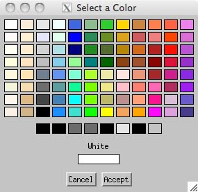
;Show color table
colorName = PickColorName(startColorName)

; Make heat map (warning, not very sophisticated)


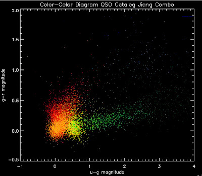
colorobject = qsotemplate1.z_sim
xobject = ugqcolor1
yobject = grqcolor1

colorbin = 0.3
colorstart = 1.0
colorstop = colorstart + colorbin

plot, xobject[0:1], yobject[0:1], ps=null, color=fsc_color('white'), xr=[-0.5,4],yr=[-0.5,2], XTITLE = 'u-g magnitude', YTITLE = 'g-r magnitude', TITLE = 'Color-Color Diagram QSO Catalog Jiang Combo', charsize = 1.5, charthick = 1

zrange = where(colorobject GE colorstart AND colorobject LT colorstop)
oplot, xobject[zrange], yobject[zrange], ps=3, color=FSC_COLOR('dark red') ;Fake QSOs
colorstart = colorstop
colorstop = colorstart + colorbin
zrange = where(colorobject GE colorstart AND colorobject LT colorstop)
oplot, xobject[zrange], yobject[zrange], ps=3, color=FSC_COLOR('red') ;Fake QSOs
colorstart = colorstop
colorstop = colorstart + colorbin
zrange = where(colorobject GE colorstart AND colorobject LT colorstop)
oplot, xobject[zrange], yobject[zrange], ps=3, color=FSC_COLOR('orange red') ;Fake QSOs
colorstart = colorstop
colorstop = colorstart + colorbin
zrange = where(colorobject GE colorstart AND colorobject LT colorstop)
oplot, xobject[zrange], yobject[zrange], ps=3, color=FSC_COLOR('orange') ;Fake QSO
colorstart = colorstop
colorstop = colorstart + colorbin
zrange = where(colorobject GE colorstart AND colorobject LT colorstop)
oplot, xobject[zrange], yobject[zrange], ps=3, color=FSC_COLOR('gold') ;Fake QSOs
colorstart = colorstop
colorstop = colorstart + colorbin
zrange = where(colorobject GE colorstart AND colorobject LT colorstop)
oplot, xobject[zrange], yobject[zrange], ps=3, color=FSC_COLOR('lawn green') ;Fake QSOs
colorstart = colorstop
colorstop = colorstart + colorbin
zrange = where(colorobject GE colorstart AND colorobject LT colorstop)
oplot, xobject[zrange], yobject[zrange], ps=3, color=FSC_COLOR('lime green') ;Fake QSOs
colorstart = colorstop
colorstop = colorstart + colorbin
zrange = where(colorobject GE colorstart AND colorobject LT colorstop)
oplot, xobject[zrange], yobject[zrange], ps=3, color=FSC_COLOR('dark green') ;Fake QSOs
colorstart = colorstop
colorstop = colorstart + colorbin
zrange = where(colorobject GE colorstart AND colorobject LT colorstop)
oplot, xobject[zrange], yobject[zrange], ps=3, color=FSC_COLOR('teal') ;Fake QSOs
colorstart = colorstop
colorstop = colorstart + colorbin
zrange = where(colorobject GE colorstart AND colorobject LT colorstop)
oplot, xobject[zrange], yobject[zrange], ps=3, color=FSC_COLOR('dodger blue') ;Fake QSOs
colorstart = colorstop
colorstop = colorstart + colorbin
zrange = where(colorobject GE colorstart AND colorobject LT colorstop)
oplot, xobject[zrange], yobject[zrange], ps=3, color=FSC_COLOR('royal blue') ;Fake QSOs
colorstart = colorstop
colorstop = colorstart + colorbin
zrange = where(colorobject GE colorstart AND colorobject LT colorstop)
oplot, xobject[zrange], yobject[zrange], ps=3, color=FSC_COLOR('blue') ;Fake QSOs
colorstart = colorstop
colorstop = colorstart + colorbin
zrange = where(colorobject GE colorstart AND colorobject LT colorstop)
oplot, xobject[zrange], yobject[zrange], ps=3, color=FSC_COLOR('navy') ;Fake QSOs
colorstart = colorstop
colorstop = colorstart + colorbin
zrange = where(colorobject GE colorstart AND colorobject LT colorstop)
oplot, xobject[zrange], yobject[zrange], ps=3, color=FSC_COLOR('dark slate blue') ;Fake QSOs
colorstart = colorstop
colorstop = colorstart + colorbin
zrange = where(colorobject GE colorstart AND colorobject LT colorstop)
oplot, xobject[zrange], yobject[zrange], ps=3, color=FSC_COLOR('dark orchid') ;Fake QSOs

The hope is that I will expand on this list every time I come across something I think I might use again (but don't use enough to memorize).

Housekeeping

I've restructured the way the code is run to that I can do multiple runs at once and to hopefully make it easier to re-produce runs and look at older runs quickly. Below is how it works.

Whenever I do a new run, the first thing that python does is create a new 'working directory' of the following format:

runYYYYMD_HM

where
YYYY is the year (2010)
M is the month (2)
D is the day (1)
H is the hour (1337)
so in this example the directory would be called: run201021_1337

This in done in python by the following code:

now = dt.datetime.now()
year = now.year
month = now.month
day = now.day
hour = now.hour
minute = now.minute
workingDir = "run%d%d%d_%d%d"%(year,month,day,hour,minute)
command = "mkdir "+ workingDir
os.system(command)

Within this directory all the photometric and spectroscopic data files are placed for each of the redshift bins. These files are in the format:

photo2D.dat - ra and dec of all photometric data
spec2D_#.dat - ra and dec of the spectroscopic data in the # redshift bin
spec3D_#.dat - x, y, z of the spectroscopic data in the # redshift bin
photoCD.dat - the comoving distance of the photometric data (from photo-zs)

I then compute the 2D cross correlation functions between the photo2D.dat and spec2D_#.dat files and these are saved in the wps#.dat files. The input arguments for these correlation functions are in the files wpsInputs#.

I then compute the 3D auto correlation functions on the spec3D_#.dat files and these are saved in the xiss#.dat files. The input arguments for these correlation functions are in the files xiInputs#.

Because the correlation functions in each redshift bin are submitted as qsub jobs, they take a while to run... so at this point you need to wait for all those jobs to finish. The jobs are named as follows:

2D Cross Correlation: JessWps#workingDir
3D Auto Correlation: JessXiss#workingDir

where # is the redshift bin and workingDir is the name of the working directory.

I can monitor the qsub jobs by typing in 'qstat' to see what is running. Once all the jobs for my working directory are completed then I do the following:

load in the constants from the run file (I put this in the working directory) and it is named YYMMDD_#run.py

where YY is the year (10)
MM is the month (02)
and DD is the day (01)
# is the run number (if I've done multiple runs on this day)

I set the variable workingDir to the working directory.

I load in the photometric comoving distances (which are saved in a file called photoCD.dat):

photoCD = readPhotoCDfile(photoCDfile)

I create the wps and xi matrixes (which are used in the reconstruction) and save them as files:

wpsMat.dat and xiMat.dat respectively.

Then I can do the reconstruction of the redshift distribution and compare it to the photoCD.

Plotting with Joe

Joe Hennawi and I worked on trying to figure out where exactly we are going wrong with the likelihood method. He suggested making a two-dimensional histogram of the likelihoods binned in color-color space. This would allow us to see where in color-color space were are getting objects which have high likelihoods and will help us debug if there is a population of objects which are being falsely selected.

It is quite easy to make the 2D histogram, but plotting it has proved to be an issue. I've spent most of the day trying to do this. Here is how I create the histogram:

qsos = testqsos

b_u = 1.4
b_g = 0.9
b_r = 1.2
b_i = 1.8
b_z = 7.4

z_temp = qsos.Z_TOT
fu1 = qsos.PSFFLUX[0]
fg1 = qsos.PSFFLUX[1]
fr1 = qsos.PSFFLUX[2]
fi1 = qsos.PSFFLUX[3]
fz1 = qsos.PSFFLUX[4]

ivar_u1 = qsos.PSFFLUX_IVAR[0]
ivar_g1 = qsos.PSFFLUX_IVAR[1]
ivar_r1 = qsos.PSFFLUX_IVAR[2]
ivar_i1 = qsos.PSFFLUX_IVAR[3]
ivar_z1 = qsos.PSFFLUX_IVAR[4]


u1 = sdss_flux2mags(fu1, b_u)
g1 = sdss_flux2mags(fg1, b_g)
r1 = sdss_flux2mags(fr1, b_r)
i1 = sdss_flux2mags(fi1, b_i)
z1 = sdss_flux2mags(fz1, b_z)

sigu = sdss_ivar2magerr(ivar_u1, fu1, b_u)
sigg = sdss_ivar2magerr(ivar_g1, fg1, b_g)
sigr = sdss_ivar2magerr(ivar_r1, fr1, b_r)
sigi = sdss_ivar2magerr(ivar_i1, fi1, b_i)
sigz = sdss_ivar2magerr(ivar_z1, fz1, b_z)

ug = u1-g1
gr = g1-r1
ri = r1-i1
iz = i1-z1

icut = where(i1 GT 19.5)

nx = 50
ny = 50
imageQSO = fltarr(nx,ny)
imageAll = fltarr(nx,ny)
imageRatio = fltarr(nx,ny)

likeQSO = qsoqlike[icut]
likeAll = qsoslike[icut]
likeRatio = likeQSO/likeAll

qsoug = ug[icut]
qsogr = gr[icut]

populate_image, imageQSO, qsoug, qsogr, weight = likeQSO
populate_image, imageALL, qsoug, qsogr, weight = likeAll
populate_image, imageRatio, qsoug, qsogr, weight = likeRatio

Now I need code to plot this histogram in color-color space with hotter colors in bins with higher likelihoods and cooler colors in bins with smaller likelihoods. Anyone have code that does this in IDL or python? Joe has some, but I'm having a hard time getting it to work.

Bad Blogger

I've been a bad blogger this past week. Apologies for not posting. I could give excuses, but that would break two of my blog rules, so I'll quit while I am ahead (or behind as it were).

Here is a summary of where I am with this darn 3D correlation function. The Sloan data is in ra/dec/redshift coordinates. However, it is easier to calculate the 3d correlation function in x-y-z comoving coordinates. So I convert the data into comoving coordinates to calculate the correlation function. However the data lives in a ra/dec/redshift space (mask) and this corresponds to a non-boxlike x-y-z space. Therefore I need to apply the mask in ra/dec/redshift for both the randoms and the data, and then convert both to x-y-z to calculate the correlation function.

But the mock data I am currently testing my 3D correlation function with is, actually in x-y-z coordinates to begin with. This is causing an issue, because I am converting it to ra/dec/redshift, which results in non-uniform data distribution in ra/dec/redshift space (because the mock data, unlike the Sloan data, is a contiguous box in x-y-z space). However the randoms are generated in uniform ra/dec/redshift space and converted to x-y-z space (to match the Sloan mask). When I compare the mock data with the randoms they don't have the same masks because of this issue:

I think what I need to do is take the mock data in x-y-z, convert it to ra/dec/redshift and then apply a mask in that coordinate system. Then convert it back to x-y-z and use those points as my data, and then apply the same mask to the randoms. This will be more similar to what I will be doing with the Sloan data and should get my data and randoms to fall in the same location on my vector space.

Idiocy

My undergraduate research adviser Dan Snowden-Ifft always told me that the best and worst thing about computers is that they always do exactly what you tell them to do. If what they are doing isn't what you expect, then it is because you told them to do something wrong. This applies to my current situation with the randoms not matching because I was in fact asking the computer to print out the wrong numbers, and so of course they didn't match. I am in idiot sometimes. Here are some nice plots of it working now:

Random Problems

My 3D correlation function matches Alexia's (to within 10^-9 -- which I assumed was rounding differences). However, when I print out the random numbers used to calculate the correlation function they stop matching halfway through the calculation (I am using the same seeds in both runs):

What is even more mysterious is that the number of random values generated is different by 10. This makes no sense because the input files for both functions are the same and both have the same number of mock data points. Do I spend time tracking down this issue, or let is go as it doesn't really effect the end result?

Precision Comparisons

I am still meticulously implementing the changes to my 3D correlation function (Xi) and constantly comparing it to the working version (Alexia's code). I haven't found where the breakdown is occuring. However, I do have some pretty plots which show how precisely these correlation functions match:

My correlation function is exactly underneath Alexia's so you can't see any distinction. I did this by seeding the random number generators the same. Below is a plot of the difference between our 3D correlation functions. Notice the 10^-9 at the top. This is due to rounding errors in the floating point numbers.

I just need to keep them working this well, while continuing to add the new geometry. Wish me luck!

Masking Difficulties

The first change I implemented to the 3D correlation function was setting up the masks in two coordinate systems. In the 2D code the mask is simply in ra and dec (because we are taking an angular correlation function in those dimensions). In the 3D code the correlation calculation is done in comoving coordinates, however the data mask is still in ra and dec because this is how we scan the sky. Therefore the continuous space that the data lives in is in ra, dec, redshift, but the space in which we are doing the correlation calculation in is x, y, z. Because we need to apply the same mask to the randoms in our correlation function as we do to the data, I need to apply a mask in ra, dec, redshift space... but then convert to x, y, z space for the calculation. I was thinking it was somewhere in this conversion where my problems were in my code. However in the first set of changes I made, I just added two masks (in the two coordinate systems) instead of one. And I got the following result:

I am really confused how my correlation function could be off by over 10 orders of magnitude by simply changing the number of input masks. I am not actually changing the values of the masks between this version of the code and the last version I plotted. Both are taking a data set which is contiguous in x, y, z, and therefore using a mask in x, y, z for the randoms and not changing yet to ra, dec, redshift space. There should not be any difference in the actual calculation. Time to revert back to "working" version and implement the masks more slowly I guess. I hate this!

So Far So Good...

I have been working on systematically changing my 2D correlation function (which matches Alexia's 2d correlation function) to a 3D correlation function (which was looking very different from Alexia's 3D). I haven't made all the changes, but of those I have made thus far, I still get matching functions:

I haven't put in the coordinate changes yet (which is the major change, and probably the root of my problem). Let this experience be a reminder to me that I shouldn't make multiple changes at once to my code.

If you are wondering why this plot of Alexia's Xi looks different than the one in the Miserable Failure post, this is because that 3D correlation function was using an older version of Alexia's code which only looks at the correlation function in a cone with a 12 degree open angle. This version of her code calculates the correlation function on the entire box.

Time for the 'State of the Department' address. Predicted summary: We are broke!

Bad Hard Variables

Apologies for the lack of posting. It is just embarrassing to post day after day "still trying to find the error in my code." I am tempted to switch back to working on the likelihood stuff because at least I might have some progress to report. However, Josh tells me that if I don't post on my blog he is forced to do his own research -- I can't disappoint my readers (all two of them).

It turns out that there were some hard-wired constants in Alexia's 2D correlation function that I forgot about. When I adjusted those for the mock catalog I got my 2D function to match hers (thank goodness something is working):

Next step is to systematically make the changes from the 2D to the 3D until it breaks. I hate debugging.

Oh, and I can't believe how much nicer it has to have a software CRYPTOcard. Thank you Josh for helping me get one!

Coordinate Confusion

Time to run my 3D autocorrelation function on a mock catalog where we know the answer to try to see if there is a problem with my code or that the reconstruction is failing for another reason. I downloaded the following raw mock LRG catalog from Martin White's web page: halo_000_0.8000.dat.gz. I discovered that I can transfer files to riemann via the insure replacement by doing a two step scp. That is useful to know.

The code I am using to convert from ra, dec (degrees), comoving distance (r) to x, y, z and back:

%  x=r*sin(pi/2-pi/180*dec)*cos(pi/180*ra);
%  y=r*sin(pi/2-pi/180*dec)*sin(pi/180*ra);
%  z=r*cos(pi/2-pi/180*dec) ;

%  r = sqrt(x^2 + y^2 + z^2)
%  dec =  90 - 180/pi*arccos(z/r)
%  ra = 180/pi*arcsin(y/sqrt(x^2 + y^2))

I am a little confused because these mock files are in Cartesian coordinates and if I convert them using the above code into ra and dec, I don't get the objects populating all of ra/dec space:

I constrained the data to be in a sphere of radius 0.5 boxsize (936.0 Mpc/h), and I would think that the ra and dec would then go from 0 to 360 and 0 to 180 respectively.

After some digging, I discovered that by using the arctan2 function I get the proper range:

%  theta = arctan2(sqrt(x^2+y^2), z)
%  phi = arctan2(x, y)

However when I try to then convert back to Cartesian I get a strange answer when I plot the original z versus the converted back z:

This is distressing!

Sources:
http://astro.uchicago.edu/cosmus/tech/code/radecz2xxyyzz.m
http://www.atlasoftheuniverse.com/cosmodis.c
http://www.math.montana.edu/frankw/ccp/multiworld/multipleIVP/spherical/body.htm
http://www.daniweb.com/forums/post860497-2.html

Python tips for the day
1) If you are getting the following error when trying to plot:

RuntimeError: Agg rendering complexity exceeded.
Consider downsampling or decimating your data

Then exit and restart your session and try again and it for some reason works. Stupid python.

2) When converting from spherical use atan2 not asin.

Lost in Translation

I've been having this problem that when I run my 3D auto-correlation function code on my laptop it runs fine, and gives me a logical result, but when I run the same code on my LBNL machine (riemann, for those who are familiar) I get a Segmentation fault and the code crashes. The code has the same inputs for both machines. The scarier thing is that when I run the code on a file with more data points, it doesn't crash on either machine.

However, I'm supposed to write about research accomplishments, so let me show the autocorrelation functions of the files that DID run:

3D auto-correlation function

2D cross-correlation function

I think the problem is that the files which are crashing have so few data points that there are some correlation bins where there are no objects separated by that distance. I am not actually sure how the code handles this. I would hope that it would just set that bin to zero, but there is quite likely a divide by zero problem going on here. Time to insert some print statements and get to the root of this.