xmpl_rv, ximat and sximat

Alexia I suggested to look at xmpl_rv (ximat) and sximat to make sure that the interpolation of the xi matrix is in the same location as the xi matrices from the data.

The results are surprising. First of all, the plot of ximat vs sximat is basically a flat line, when plotted log space (click on images to enlarge):

The above plot has sximat, ximat for 3 different binnings (39, 40, and 41) and the plots basically all fall on top of each other. This is from the best "working" reconstruction mock data, described here.

But they don't fall on top of the xi correlation functions from the data:

I thought maybe this was a conversion issue, but I checked and I think they are in the same units. In order to even get the cximat to fall on top of the xi correlation functions you need to divide by 10^4:

Alexia am I doing this right? Is this weird to you?

Computing Time

One interesting thing I've realized in trying to compare the 2D auto-correlation with the 3D auto-correlation (on the same files) is that the 2D auto-correlation takes MUCH longer to compute than the 3D. This is strange because in this test they are computing the same number of pairs, well barring some differences in the gridding. I must be doing something very inefficient with the 2D calculation, or measuring pairs out to much larger distances than in the 3D case. The 3D auto-correlation function took less than a minute to compute, and the 2D auto-correlation function is still running, and it's been 51 minutes.

Here are the 2D and 3D autocorrelation functions on the whole set (on big redshift bin)

Below is the 3D and 2D autocorrelation on a smaller (100Mpc/h) redshift bin:

At redshift (well actually comoving distance 350 Mpc/h), what are these angular separations in Mpc/h?

What noise levels would be expect just from shot noise?

How do we expect the slopes to compare?

I talked to David, Eric, Nic and Matt about this. They gave me some references to check out and also suggested that (just as a check) I set the redshifts of the 3d correlation function to all be the same, and then calculate the 3D and 2D, and compare them, they should basically be the same then, or at least proportional to each other.

David also suggested (as a way to figure out where my troubles are coming from.... to go back to the mocks, when the reconstruction was working)... and to then try applying the BOSS Geometry to these mocks and see if I can get the code to work on the mocks with the BOSS Masks. Then once that is working, swap in the BOSS data.

It's worth a try!

References to read:

Dodelson

Peebles 1980

Limber 1954

Still need to do the binning experiments that Alexia suggested. So much to do, so few hours in the day.

Comparing Correlation Functions

I've been trying to figure out why my 2d Correlation Functions look weird. I've put out request to several Berkeley folks to compare my correlation function results on a data set with theirs, but while I wait for them to respond, I'm going to compare to some literature.

For the 2-d angular correlation function on SDSS LRG galaxies, I have the following plots from Connolly et al (2001):



And from Ross et al (2007):


I changed the angular bins of my correlation function to match these sets to try to form a comparison. Here is my 2D correlation function on BOSS data:

As you can see the slope of the function is much shallower for my correlation function, than it is the literature.

The 3D correlation functions are a better match:
From Ross et al (2007):

And here is mine:

At least the slopes seem to be comparable.

I am currently running the 3D correlation function on a larger los range to try to compare to Kazin et al. :

This will take a bit because I am correlating out to such large scales (180 Mpc/h).

Another thing I noticed that I wanted to talk to Alexia about is the actual computation of the correlation function in the code. Right now it is the following:

xi = (dd - dr - rd + rr)/rr

where

dd = # of data-data pairs in bin
dr = (# if data-random pairs in bin) / (Random Oversampling)
rd = (# if data-random pairs in bin) / (Random Oversampling)
rr = (# if random-random pairs in bin) / (Random Oversampling)

I am wondering if the rr should be divided by (random oversampling)^2 because there are that many more point in the RR set. I haven't changed this code from when I first got it from Alexia, so I assume it is correct. But I was looking the Landy, Szalay Paper and it seemed like they were using factors of n(n-1)/2 which is approximately n^2, and we are using factors of n.

Thoughts?

3/21 5:15 Update: Here is my plot of the 3d Correlation function on the large los range, it looks very similar to the Kazin plot above, you can even see the BAO signal @ ~100 Mpc/h:

At Los Alamos

I am visiting Alexia at Los Alamos National Lab for the next three weeks. Los Alamos is beautiful, but COLD.

I'm putting the final touches on the data-correlation function setup.

I noticed that in the 3D auto-correlation, I am producing two different random catalogs and using the following calculation:

(dd -dr1 -r2d +r1r2)/(r1r2)

This might be extra computing power than necessary if it is ok for r1 = r2... but I forget if they need to be different... perhaps they do need to be different in order for this to work. It seems like this is something I would have thought of before.

I talked to Alexia about this and she thinks it shouldn't make a difference either way. So I am going to set r1 = r2 and see what happens....

Old Autocorrelation Function results (without randoms fed in)
# r (Mpc/h) cross xi (r)
# r (Mpc/h) cross xi (r)
1.0009750000 113.0999999998
3.0009250000 4.3312368973
5.0008750000 0.1890557940
7.0008250000 0.3768587361
9.0007750000 0.4359240581
11.0007250000 0.1349752029
13.0006750000 0.1273595140
15.0006250000 -0.1351841518
17.0005750000 0.2378351539
19.0005250000 0.2994336370
21.0004750000 -0.0479553597
23.0004250000 -0.0998846930
25.0003750000 -0.1438266200
27.0003250000 -0.3070417433
29.0002750000 -0.3108741254
31.0002250000 -0.1177777522
33.0001750000 -0.0633376228
35.0001250000 -0.2604527820
37.0000750000 -0.2517495550
39.0000250000 -0.0304629134


New Autocorrelation Function results (with randoms fed in)
I think small differences are rounding errors
# Reached checkpoint 4
# r (Mpc/h) cross xi (r)
1.0009750000 113.0999999998
3.0009250000 4.3294918806
5.0008750000 0.1890963726
7.0008250000 0.3766263941
9.0007750000 0.4359240581
11.0007250000 0.1349752029
13.0006750000 0.1273650408
15.0006250000 -0.1355281973
17.0005750000 0.2380827199
19.0005250000 0.2995001354
21.0004750000 -0.0479749624
23.0004250000 -0.0998864926
25.0003750000 -0.1437953465
27.0003250000 -0.3070974753
29.0002750000 -0.3107744869
31.0002250000 -0.1177689518
33.0001750000 -0.0632545877
35.0001250000 -0.2605975485
37.0000750000 -0.2517029624
39.0000250000 -0.0304363094

New Autocorrelation Function with r1 = r2 (with randoms fed in)
There are pretty big difference between these two, but this could just be because my data set is small. Should check on a larger set.
# Reached checkpoint 4
# r (Mpc/h) cross xi (r)
1.0009750000 120.9999999998
3.0009250000 3.9579487179
5.0008750000 0.1234024722
7.0008250000 0.3826803206
9.0007750000 0.4731333382
11.0007250000 0.0871628790
13.0006750000 0.0808080808
15.0006250000 -0.1168749344
17.0005750000 0.2334021835
19.0005250000 0.3148748159
21.0004750000 -0.0339674194
23.0004250000 -0.0762365727
25.0003750000 -0.1365716955
27.0003250000 -0.2876355988
29.0002750000 -0.3209356312
31.0002250000 -0.1164599148
33.0001750000 -0.0517181534
35.0001250000 -0.2402264337
37.0000750000 -0.2732306595
39.0000250000 -0.0168706759

Modifying 3D Correlation Function

I'm changing the 3D correlation function code to accept data and randoms (similar to what I just did for the 2D correlation function code).

This is proving to be a little tricky because in the current version I do some tricks to make sure the periodic boundary conditions don't add power incorrectly, and I also re-scale the data because the correlation function is expecting it to be in a 1X1X1 box.

After talking with Alexia, I've decided to do these conversions outside of the correlation function in python, such that the code expects the data to be in a 1x1x1 box.

Results to come soon.....

Changing 3D Correlation Function

One of my "things to think about" from yesterday's blog post was to make changes to the 3D correlation function so that it was truly an auto-correlation (only having one set of randoms which should speed up the calculation by a bit).

I made changes to my 3D correlation function to do this (at least I think I have) and I am running a test to see if I get the same solution as when I have two separate random catalogs (what I was doing) and also to see how much this speeds things up.

This set of runs in in the working directory: ../pythonjess/run201048_1527 and the log file where the code to run this is ../logs/100408log.py.

The new version runs in 7 seconds, whereas before it took 20 seconds! So that is a good improvement.

Here is a plot to show they look the same

Buzz Comments from Erin about qsub and splitting up the jobs:

Erin Sheldon - Have you used the PBS system on riemann? You can submit jobs and they get sent to different machines on the system. You could split your random runs into 25 different jobs, run them in parallel on 25 different machines, and then just add up the counts later.

That's a factor of n_machines speedup, better than you could every hope to get by just writing faster code.

Below is a sample script, let's call it test.pbs. You can submit with "qsub test.pbs". Of course change all the log file paths to make sense for you.
Erin

#PBS -l nodes=1:ppn=1
#PBS -l walltime=24:00:00
#PBS -q batch
#PBS -N this_job_name
#PBS -j oe
#PBS -o /path/to/where/the/pbs/script/is/test.pbs.pbslog
#PBS -m a
#PBS -V
#PBS -r n
#PBS -W umask=0022

# put setups here

setup numpy -r ~esheldon/exports/numpy-trunk
setup scipy -r ~esheldon/exports/scipy-trunk
setup esutil -r ~esheldon/exports/esutil-trunk
setup python -r ~esheldon/exports/python/2.6.4

# this log is different than above, you can
# watch it in real time
logfile=/path/to/where/the/pbs/script/is/test.pbs.log

# send commands to python
python &> "$logfile" <6:49 amDeleteUndo deleteReport spamNot spam

Erin Sheldon - oh, and to see the status of your jobs
qstat -n -1 -u your_user_name

or equivalently:
~esheldon/python/bin/pbswatch6:55 am

Speeding-up the Correlation Function

I ran another comparison between Sheldon's and my correlation function on a larger data set. Erin had suggested that I play with the depth (this is something to do with the grid spacing of his function). Below is an email from him:

So the default depth of the tree is depth=10. It seems that a lower depth, and thus lower resolution, is better for these very large 10-degree search angles. Here are some timing numbers that show depth=6 is best. You would do this to set your depth:

h=esutil.htm.HTM(depth)
depth seconds
3 137.153673172
4 114.97971487
5 104.600896835
6 99.5818519592
7 102.73042202
8 119.931453943
9 185.077499866
10 460.641659021
11 1502.35429096

Erin also thinks I am correlating out to too large of an angle. Alexia did a quick calculation and agrees with this assessment. This is another reason why my correlation functions are taking so long. Erin suggests that I try working in physical space (Mpc) instead of angular space:

Another thing to try is working in physical space. 10 degrees is definitely too large in angle. If you are, for example, willing to work at 30Mpc you could get big speedups. You know the redshifts of the spectroscopic sample of course. So you just bin in physical projected separation as defined by:

d*angle

where d is the angular diameter distance in Mpc and angle is in radians. The bincount function is set up to do this. If you send the scale= keyword then the rmin,rmax arguments will be in units of the scale*angle.

Let's say you have the spectroscopic sample. ra1, dec1, z1 And the second sample is the photometric sample. ra2,dec2

# you can also give omega_m etc. here, see docs
cosmo = esutil.cosmology.Cosmo()

# get angular diameter distance
# to points in set 1
d = cosmo.Da(0.0, z1)

rmin = 0.025 # Note units in Mpc
rmax = 30 # Mpc
nbin = 25

rlower,rupper,counts = h.bincount(rmin,rmax,nbin,ra1,dec1,ra2,dec2,scale=d)

Now rlower,rupper are also in Mpc.

I did a bigger run on 356,915 objects out to 10 degrees, here are the numbers:

For Erin's
Start time = 12:59:24.71
End time = 13:32:24.96
Run time = 1980.25 seconds ≈ 33 minutes

For Mine
Start time = 12:57:33.83
End time = 13:40:35.13
Run time = 2581.30 seconds ≈ 43 minutes

A few things to think about:

• Should I change the correlation angle as a function of the spectroscopic redshift? Can the reconstruction handle this?
• I am currently running the DD, DR, RD, RR correlations all in succession, but they could be run simultaneously and this could in theory speed up the calculation.
• What are the correct angles and comoving distances I should be correlating out to? Obviously going out to 20 degrees is too much. Alexia's quick calculations estimates that I only need to go out to 6 degrees, but this varies with redshift.
• Sheldon's code does run faster and has more functionality. Should I use it from now on?
• The 3D correlation function is always an auto-correlation function, and so there is no need to calculate both DR and RD and so I could change this code to run faster by calculating the correlation as DD - 2DR + RR. Of course RR is going to be 25X more points that DD and 5X as DR (I am over sampling by 5) so most the time of the calculation is spent there.

Plot

Happy Birthday Toni and Cleo

Data Run

I'm running the reconstruction on the data. I'm doing in the working directory: .../pythonJess/run2010329_1319. I am running this with 12 redshift bins and 250k photometric and spectroscopic objects.

I did a little bit of thinking about the number of grids for the correlation function. There is the strange balance that you want the number of grids to be less than the number of particles, otherwise you might as well just correlate all possible pairs. You also want the spacing to be much bigger than the max correlation length, otherwise even by going out one grid length, you will unnecessarily correlate too many objects. I feel like this is a computer science problem, and perhaps Adam Pauls or Erin Sheldon would know the answer?

I played with this a bit (tried upping the grid points to 1000, and this took forever to run). For the 2D correlation function, I am correlating out to a distance of 0.34 (with a box size of 1). Maybe I don't need to correlate out to such a big angle? We could probably have as few as 10 grid points in each dimension if we are going out to this large of an angle. For the 3D correlation function, I am correlating out to a distance of 20 Mpc/h (with a box size of 2400 Mpc/h) so we need at least ~120 grid points in each dimension.

For the 3D correlation function, some of the larger redshift bins have very few objects in them, and if we have ~100³ or 10⁶ grid points then we are wasting time griding if we have less than 10³ points in each set.

Here are the results from the reconstruction I ran yesterday. It looks like I don't have enough points because the correlation functions are very noisy.

The reconstructions don't look good and are highly variable:

I'm running on a bigger data set now.

If It Isn't One Correlation Function, It's Another!

I ran my code on the Stripe-82 data for the first time since I fixed the angular correlation functions and now my 3D correlation functions look weird:

I think this has something to do with some changes I made to the conversion from ra/dec to x, y, z. I had been doing something that I don't think is right before and I changed that, but it might now be messing up the masks so that my mask for the 3D correlation functions are now not in the same region as the data. I'm going back to look at the changes I made to investigate this. Thank goodness for repositories!

Back on Track

I fixed the angular correlation function using the method outlined in my last post. I did a run again on the mock data using photometric and spectroscopic sets with 200,000 objects. The correlation functions look much better now (and the code runs much faster too!):

2D and 3D correlation functions

The 2D are actual angular separations (different from what Alexia was doing which was collapsing the third dimension onto a projection plane). This is super exciting because the noise has gone down a lot compared to what I was getting before. Hopefully this will mean a better reconstruction.

The distribution functions I applied to the two data sets are below:

The cyan line is a histogram of the number photometric objects as a function of comoving distance away from the observer. The magenta line is the imposed photometric distribution function (what we are trying to reconstruct). The green line is a histogram of the number of spectroscopic objects as a function of comoving distance away from the observer. Note that it is different than the photometric distribution.

And here is the reconstruction:

The magenta is the imposed distribution function (same as the previous plot) and the red is the reconstructed distribution. They look pretty much the same. Awesome.

1M Reconstruction

I ran a big reconstruction on the CAS data using 1,000,000 objects, and 20 redshift bins. The correlation functions at the lower redshifts (less than 720 Mpc/h) have much less noise:


But the correlation functions at larger redshifts look pretty noisy:

Perhaps I should bin so that I have a constant number of objects per bin instead of by equal redshift bins.

When I do the reconstruction, I get puzzling results:

The reconstruction seems to think there are a large number of points at redshift > 1.0 which aren't there. This could be due to low statistics at these redshifts and so the reconstruction just isn't working properly. The number of spectroscopic objects per bin is as follows:

0-120 Mpc/h: 14597 galaxies in spectroscopic dataset
120-240 Mpc/h: 45954 galaxies in spectroscopic dataset
240-360 Mpc/h: 55489 galaxies in spectroscopic dataset
360-480 Mpc/h: 59451 galaxies in spectroscopic dataset
480-600 Mpc/h: 64381 galaxies in spectroscopic dataset
600-720 Mpc/h: 56290 galaxies in spectroscopic dataset
720-840 Mpc/h: 55916 galaxies in spectroscopic dataset
840-960 Mpc/h: 49536 galaxies in spectroscopic dataset
960-1080 Mpc/h: 29109 galaxies in spectroscopic dataset
1080-1200 Mpc/h: 20852 galaxies in spectroscopic dataset
1200-1320 Mpc/h: 16729 galaxies in spectroscopic dataset
1320-1440 Mpc/h: 13715 galaxies in spectroscopic dataset
1440-1560 Mpc/h: 8969 galaxies in spectroscopic dataset
1560-1680 Mpc/h: 5094 galaxies in spectroscopic dataset
1680-1800 Mpc/h: 2374 galaxies in spectroscopic dataset
1800-1920 Mpc/h: 890 galaxies in spectroscopic dataset
1920-2040 Mpc/h: 381 galaxies in spectroscopic dataset
2040-2160 Mpc/h: 169 galaxies in spectroscopic dataset
2160-2280 Mpc/h: 85 galaxies in spectroscopic dataset
2280-2400 Mpc/h: 16 galaxies in spectroscopic dataset

It looks like I shouldn't use bins greater than ~1Mpc/h for the reconstruction because we have so few galaxies out there. If I try doing the reconstruction only using bins up to 1080 Mpc/h this is that I get:

There seems to be a problem at the earlier redshifts, perhaps due to low statistics in the first redshift bin? But the reconstruction looks sort of good.

I'm need to see what Alexia thinks about this "forcing to zero" issue at the edges. I also want to try this with the LRG catalog. I'm going to set a run going where I bin such that there are constant numbers of galaxies per bin, not constant redshifts. Alexia, let's chat tomorrow early?

Changing Bins

After struggling with a segmentation fault problem, I have run the reconstruction with different bins. The 3D correlation functions seem to be having some problems at small separations (see plot below), need to look into this. The reconstruction still looks ok, although it seems to be very dependent on how many phi bins I use to reconstruct (see Playing with Reconstruction post). I need to get to the bottom of this. Next step, seeing what it looks like on the CAS data.

Mock Reconstruction

I ran a full reconstruction on the mock data over the past couple days. There are some problems with this run (which I discovered after I started it running, but decided to just let it finish). The first is that I have not fixed the distribution of the randoms in the 2D correlation function to go as cosine for the declinations (they are flat). The second is that I discovered the mock catalog I was using was not dark matter halos but actually LRGs and to the clustering properties are nonsensical. I have since gotten a dark matter halo catalog from Martin White.

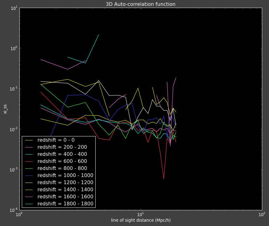
Here are the 2D and 3D correlation function for the various redshift bins:

2D correlation functions for redshift bins


3D correlation functions for redshift bins

As you can see the 3D correlation function are no longer fluctuating around zero as they were on the Sloan data.

The reconstruction is a bit puzzling. Below is a histogram of the comoving distances (from the center of the sphere) of the spectroscopic (yellow), photometric (green) data sets as well as the reconstructed phi (redshift distribution (pink)). You will noticed that while the histograms don't match, the bumps in the photometric/spectroscopic histograms seem to match the bumps in phi. I was thinking that because these photometric/spectroscopic histograms include both the geometry and the "selection function" so to speak (I didn't actually apply a selection function, so it is just the natural clustering of the objects). Whereas phi (I think) is only supposed to be the selection function, not the geometry. I was wondering if perhaps if I subtract the geometry from the p/s histograms (which is proportional to r^2) then we would basically be left with these same wiggles? I've asked Alexia about this and I am waiting for a response.

Catalog Woes

It turns out my mock catalog is probably not what I want to be using. I talked to Alexia and Martin White, and I am using a LRG catalog, but I want to be using a halo catalog. This probably means that my clustering properties are nonsensical (because I am generating galaxies based on galaxies, not on halos). Martin said he is going to give me a better catalog to use.

In the mean time I am running on the catalog I have. The reconstruction should work as long as both the photometric and spectroscopic data sets are generated in the same way... even if they don't accurately represent any real distribution on the sky.

The reconstruction is currently running, and I should have it done later today.

I also checked my 3D slice against Alexia's to make sure they match, and they do:

My and Alexia's 3D Correlation functions on
a redshift slice of the mock data

Degrees vs. Radians

Turns out the "List length exceeded MaxList" error was due to the randoms not falling in the same region as the data. I had forgotten to convert my data from radians to degrees in Python (but it was being converted in the C program) and so the C-converted randoms (in x, y, z) did not match the Python-converted data (in x, y, z).

I've fixed this, and get the following 3D correlation functions for my redshift slices of the Mock data (and they look pretty darn good)!

My 3D Correlation function on Mock Data

This makes me want to make the bold statement that all the problems I was having with my 3D correlation functions on the Sloan data was a problem with the data, (not my code)... but I need to check this again because the 2D correlation functions looked ok on the Sloan data. This could be an issue of the photo-z's just being completely wrong, (David keeps saying he doesn't trust the CAS) so the 2D correlation function (which only uses ra and dec) is fine, but once we start using the photo-z's things get messed up.

Another thought I had was that I need to fix this declination random cosine population issue in the 2D correlation function, currently the declinations are being populated using a flat distribution.

Oh today is a good day indeed!

Exceeded Maxlist

I am getting a strange error when I run the 3D Correlation function. The error is from Martin White's meshing algorithm (nearmesh):

"List length exceeded MaxList=234700"

It think it happens when a point is near any mesh within the grid. But I am not sure exactly, I didn't write this section of the code, and I've never gotten this error before.

I wrote Alexia about it, and I am hoping she'll have some experience with this problem.

Below is the email I send her today:

-------
From: Jessica Ann Kirkpatrick
Date: Tue, Nov 17, 2009 at 11:24 PM
Subject: halo files and numbers
To: Alexia Schulz

Alexia,
the file I am using is from here: http://mwhite.berkeley.edu/Mock/

It was under a section that used to be there called LRG but now seems to be gone. See this blog entry.

The number of halos in the file is 102496.

When I run halolist with mmin = 5e10 I get 3811293 galaxies (for photometric data set)
When I run halolist with mmin = 5e11 I get 378932 galaxies (for spectroscopic data set)

output when I run halolist is below:

In [324]: #make galaxies
In [325]: mmin=5.e10 #for gal
In [326]: h=gals.halolist(mockLRGfile,mmin)
1.30144190788 seconds wall time to readin
1.3 seconds processor time to readin
33.0253970623 seconds wall time
30.84 seconds processor time

In [327]: g=gals.galist(h,nbins,outfile=photofile)
4.70264683703
halo number is 102496
number of halos with 1 or more gals 102496
176.569406033 seconds wall time
168.58 seconds processor time

In [328]: mmin=5.e11 #for spec
In [329]: h=gals.halolist(mockLRGfile,mmin)
10.7454509735 seconds wall time to readin
1.66 seconds processor time to readin
37.9757530689 seconds wall time
27.46 seconds processor time

In [330]: g=gals.galist(h,nbins,outfile=specfile)
4.70264683703
halo number is 102496
number of halos with 1 or more gals 101718
27.7532730103 seconds wall time
26.72 seconds processor time

I'm getting the error:
List length exceeded MaxList=234700
on one of my runs, has this ever happened to you?

It seems to be coming from deep in the calculation in the function meshnear.

I am getting this error when I try to run on redshift slices which are further away (and thus have higher statistics).

Tomorrow the BigBOSS meeting has a break from 12-1. Can I call you sometime in that window?
Cheers,
Jessica

--------

I thought perhaps a problem is that the randoms are not overlaping with the data (and so the nearmesh would mess up because the randoms are not in the same region as the data).

And this seems to be part of the problem:

Need to check these to see where the problem is. I think there might be a degrees vs radians issue. I'll look at this tomorrow.

Mock Slice

The next step in trying to figure out what is wrong with my 3D correlation functions is to try to actually do a full reconstruction on the mock data. I'm starting with taking a redshift slice of the mock data and calculating a 3D correlation function on the slice to see if I get a logical result. This appears to be working:

Matching 3D correlation functions

To be more explicit about what I am doing to create the above. I am first taking the mock data box and selecting a "redshift slice" of the data:

For my correlation function:

Redshift slice (green) of all data points in
comoving distance range of 350-450 Mpc/h

What this looks like in Cartesian coordinates:

It is hard to see in 2D projections,

but this is essentially a thick spherical shell with inner radius
350 Mpc/h and outer radius 450 Mph/h

For Alexia's correlation function I am taking a slice in the z dimension:

Redshift slice (green) for Alexia's data

I chose the slice such that both mine and Alexia's data subsets had approximately the same number of objects (~100,000).

The distributions of the randoms continue to match the data:
For my correlation function:

Number of randoms (blue) and data points (red)
for different dimensions (ra, dec, redshift, x, y, z)

This gives me the confidence to try to do the full reconstruction on this mock data set, as that would simply be just repeating the above on several redshift bins.

I seem to be running Alexia's and my correlation functions side by side a lot to compare the results, I have made the following scripts:

svn +x *.script
./091105jess.script 091105jess.out 2> 091105jess.err &
./091105alexia.script 091105alexia.out 2> 091105alexia.err &

Cool link of the day:
Now my parents can understand xkcd: http://www.explainxkcd.com/

Update (from Kevin):
As far as http://www.xkcd.com is concerned,
http://www.explainxkcd.com is useful,
but http://xkcdexplained.com/ is funny,
and http://xkcdexplainedexplained.tumblr.com/ exists.