Computing Time

One interesting thing I've realized in trying to compare the 2D auto-correlation with the 3D auto-correlation (on the same files) is that the 2D auto-correlation takes MUCH longer to compute than the 3D. This is strange because in this test they are computing the same number of pairs, well barring some differences in the gridding. I must be doing something very inefficient with the 2D calculation, or measuring pairs out to much larger distances than in the 3D case. The 3D auto-correlation function took less than a minute to compute, and the 2D auto-correlation function is still running, and it's been 51 minutes.

Here are the 2D and 3D autocorrelation functions on the whole set (on big redshift bin)

Below is the 3D and 2D autocorrelation on a smaller (100Mpc/h) redshift bin:

At redshift (well actually comoving distance 350 Mpc/h), what are these angular separations in Mpc/h?

What noise levels would be expect just from shot noise?

How do we expect the slopes to compare?

I talked to David, Eric, Nic and Matt about this. They gave me some references to check out and also suggested that (just as a check) I set the redshifts of the 3d correlation function to all be the same, and then calculate the 3D and 2D, and compare them, they should basically be the same then, or at least proportional to each other.

David also suggested (as a way to figure out where my troubles are coming from.... to go back to the mocks, when the reconstruction was working)... and to then try applying the BOSS Geometry to these mocks and see if I can get the code to work on the mocks with the BOSS Masks. Then once that is working, swap in the BOSS data.

It's worth a try!

References to read:

Dodelson

Peebles 1980

Limber 1954

Still need to do the binning experiments that Alexia suggested. So much to do, so few hours in the day.

Matching Angular Correlation Function

After banging my head against my code for a while, I seem to finally have a 2d correlation function result that matches the literature....

Published result (from Ross 2007):

Mine:

The values match!

This is an autocorrelation. I want to make sure it doesn't change significantly when I do a cross correlation, then I am going to try and see how it looks when I run in on several bins.

Min

Comparing Correlation Functions

I've been trying to figure out why my 2d Correlation Functions look weird. I've put out request to several Berkeley folks to compare my correlation function results on a data set with theirs, but while I wait for them to respond, I'm going to compare to some literature.

For the 2-d angular correlation function on SDSS LRG galaxies, I have the following plots from Connolly et al (2001):



And from Ross et al (2007):


I changed the angular bins of my correlation function to match these sets to try to form a comparison. Here is my 2D correlation function on BOSS data:

As you can see the slope of the function is much shallower for my correlation function, than it is the literature.

The 3D correlation functions are a better match:
From Ross et al (2007):

And here is mine:

At least the slopes seem to be comparable.

I am currently running the 3D correlation function on a larger los range to try to compare to Kazin et al. :

This will take a bit because I am correlating out to such large scales (180 Mpc/h).

Another thing I noticed that I wanted to talk to Alexia about is the actual computation of the correlation function in the code. Right now it is the following:

xi = (dd - dr - rd + rr)/rr

where

dd = # of data-data pairs in bin
dr = (# if data-random pairs in bin) / (Random Oversampling)
rd = (# if data-random pairs in bin) / (Random Oversampling)
rr = (# if random-random pairs in bin) / (Random Oversampling)

I am wondering if the rr should be divided by (random oversampling)^2 because there are that many more point in the RR set. I haven't changed this code from when I first got it from Alexia, so I assume it is correct. But I was looking the Landy, Szalay Paper and it seemed like they were using factors of n(n-1)/2 which is approximately n^2, and we are using factors of n.

Thoughts?

3/21 5:15 Update: Here is my plot of the 3d Correlation function on the large los range, it looks very similar to the Kazin plot above, you can even see the BAO signal @ ~100 Mpc/h:

Princeton Progress

We have some confusing findings from this week. First of all, I re-ran the reconstruction on a smaller angular scale (as both Alexia and Erin told me to do as I was going out to way to large of scales) and got the following for the angular correlation functions:

Close up on a few:

This concerns Alexia and me because first of all they are almost featureless on this degree scale (they look really flat). Second, they seem to move in the wrong direction as a function of redshift bin. We would expect that as we go out further in redshift, the same angular separation would correspond to larger physical separation of objects, and thus the angular correlation should decrease as redshift increases (see below), but we are seeing the opposite.

From Connolly et al. arXiv:astro-ph/0107417v2

Here are the 3D correlation functions:

Here are the photometric and spectroscopic redshift distributions

And the best fit reconstruction, which isn't very good

And I am still getting problems with changing the binning dramatically influencing the reconstruction.

List of things to do:
1. Run my angular correlation function on the same data set as in this paper, and see if I get the same solution.
2. Alexia is running the reconstruction on her data sets to see if she gets the same strange behavior for the correlation functions as a function of redshift.
3. Alexia is going to play with the binning and see if she gets the same strange behavior.
4. I need to come up with another way to do the reconstruction that doesn't involve this lambda/tolerance but minimizes the ximat...

Speeding-up the Correlation Function

I ran another comparison between Sheldon's and my correlation function on a larger data set. Erin had suggested that I play with the depth (this is something to do with the grid spacing of his function). Below is an email from him:

So the default depth of the tree is depth=10. It seems that a lower depth, and thus lower resolution, is better for these very large 10-degree search angles. Here are some timing numbers that show depth=6 is best. You would do this to set your depth:

h=esutil.htm.HTM(depth)
depth seconds
3 137.153673172
4 114.97971487
5 104.600896835
6 99.5818519592
7 102.73042202
8 119.931453943
9 185.077499866
10 460.641659021
11 1502.35429096

Erin also thinks I am correlating out to too large of an angle. Alexia did a quick calculation and agrees with this assessment. This is another reason why my correlation functions are taking so long. Erin suggests that I try working in physical space (Mpc) instead of angular space:

Another thing to try is working in physical space. 10 degrees is definitely too large in angle. If you are, for example, willing to work at 30Mpc you could get big speedups. You know the redshifts of the spectroscopic sample of course. So you just bin in physical projected separation as defined by:

d*angle

where d is the angular diameter distance in Mpc and angle is in radians. The bincount function is set up to do this. If you send the scale= keyword then the rmin,rmax arguments will be in units of the scale*angle.

Let's say you have the spectroscopic sample. ra1, dec1, z1 And the second sample is the photometric sample. ra2,dec2

# you can also give omega_m etc. here, see docs
cosmo = esutil.cosmology.Cosmo()

# get angular diameter distance
# to points in set 1
d = cosmo.Da(0.0, z1)

rmin = 0.025 # Note units in Mpc
rmax = 30 # Mpc
nbin = 25

rlower,rupper,counts = h.bincount(rmin,rmax,nbin,ra1,dec1,ra2,dec2,scale=d)

Now rlower,rupper are also in Mpc.

I did a bigger run on 356,915 objects out to 10 degrees, here are the numbers:

For Erin's
Start time = 12:59:24.71
End time = 13:32:24.96
Run time = 1980.25 seconds ≈ 33 minutes

For Mine
Start time = 12:57:33.83
End time = 13:40:35.13
Run time = 2581.30 seconds ≈ 43 minutes

A few things to think about:

• Should I change the correlation angle as a function of the spectroscopic redshift? Can the reconstruction handle this?
• I am currently running the DD, DR, RD, RR correlations all in succession, but they could be run simultaneously and this could in theory speed up the calculation.
• What are the correct angles and comoving distances I should be correlating out to? Obviously going out to 20 degrees is too much. Alexia's quick calculations estimates that I only need to go out to 6 degrees, but this varies with redshift.
• Sheldon's code does run faster and has more functionality. Should I use it from now on?
• The 3D correlation function is always an auto-correlation function, and so there is no need to calculate both DR and RD and so I could change this code to run faster by calculating the correlation as DD - 2DR + RR. Of course RR is going to be 25X more points that DD and 5X as DR (I am over sampling by 5) so most the time of the calculation is spent there.

Plot

Happy Birthday Toni and Cleo

Comparing Correlation Function

I ran a simple experiment to compare Erin Sheldon's correlation function and mine/Alexia's. I modified my correlation function so that it was only calculating the data-data pair counts. I did the same with Erin's. I did this on a set of 53,071 objects. I did an auto-correlation for simplicity (both data sets were the same).

For Erin's
Start time = 16:01:53:98
End time = 16:09:11:49
Run time = 437.51 seconds

For Mine
Start time = 16:24:27:99
End time = 16:26:12:03
Run time = 104.04 seconds

The number of pair counts match pretty well, except for at the ends which I believe is just a binning effect:

I'm kind of confused why my correlation function is 4X faster on this data set, when ball-park numbers Erin and I were comparing before implied that his should run much faster. I am going to see if maybe they scale differently with number of points by running on a larger data set.

Sheldon's Correlaton Function

Erin Sheldon is helping me with my 2D correlation function. He has one that runs a lot faster than the one I have been using. He has been amazing in helping me to get it working with my data set.

After some incompatibility problems with various packages we needed for running our respective code it seems to be able working now (well it compiles and passes the checks). However, when I try to run it I get the following error:

RuntimeError: found log_binsize < 0

I've pinged Erin about this, so we'll see if he has ideas. The code I'm using to test this is in the following log file: .../logs/100405log.py

7:15 Update: Erin Rocks! He just got back to me with a fix. It is running now! I'm going to do some tests to see how long it takes and compare it's answer with my correlation function's answer.

Outputs:
Generating HTM ids
Generating reverse indices
rmin: 0.001
rmax: 10
degrees?: True
nbin: 25
logrmin: -3
logrmax: 1
log binsize: 0.16
len(scale_array) = 0

Each dot is 500 points
......................................................................
35000/53071 pair count: 176696860
....................................

In [15]: rlower
Out[15]:
array([ 1.00000000e-03, 1.44543977e-03, 2.08929613e-03,
3.01995172e-03, 4.36515832e-03, 6.30957344e-03,
9.12010839e-03, 1.31825674e-02, 1.90546072e-02,
2.75422870e-02, 3.98107171e-02, 5.75439937e-02,
8.31763771e-02, 1.20226443e-01, 1.73780083e-01,
2.51188643e-01, 3.63078055e-01, 5.24807460e-01,
7.58577575e-01, 1.09647820e+00, 1.58489319e+00,
2.29086765e+00, 3.31131121e+00, 4.78630092e+00,
6.91830971e+00])

In [16]: rupper
Out[16]:
array([ 1.44543977e-03, 2.08929613e-03, 3.01995172e-03,
4.36515832e-03, 6.30957344e-03, 9.12010839e-03,
1.31825674e-02, 1.90546072e-02, 2.75422870e-02,
3.98107171e-02, 5.75439937e-02, 8.31763771e-02,
1.20226443e-01, 1.73780083e-01, 2.51188643e-01,
3.63078055e-01, 5.24807460e-01, 7.58577575e-01,
1.09647820e+00, 1.58489319e+00, 2.29086765e+00,
3.31131121e+00, 4.78630092e+00, 6.91830971e+00,
1.00000000e+01])

In [17]: counts
Out[17]:
array([ 468, 512, 758, 1216, 2176, 4266,
6962, 13332, 25388, 46232, 83912, 146620,
246088, 377354, 523490, 674092, 972164, 1683416,
3167032, 6144742, 12083396, 22744048, 41867790, 71782726,
105281816])

Data Run

I'm running the reconstruction on the data. I'm doing in the working directory: .../pythonJess/run2010329_1319. I am running this with 12 redshift bins and 250k photometric and spectroscopic objects.

I did a little bit of thinking about the number of grids for the correlation function. There is the strange balance that you want the number of grids to be less than the number of particles, otherwise you might as well just correlate all possible pairs. You also want the spacing to be much bigger than the max correlation length, otherwise even by going out one grid length, you will unnecessarily correlate too many objects. I feel like this is a computer science problem, and perhaps Adam Pauls or Erin Sheldon would know the answer?

I played with this a bit (tried upping the grid points to 1000, and this took forever to run). For the 2D correlation function, I am correlating out to a distance of 0.34 (with a box size of 1). Maybe I don't need to correlate out to such a big angle? We could probably have as few as 10 grid points in each dimension if we are going out to this large of an angle. For the 3D correlation function, I am correlating out to a distance of 20 Mpc/h (with a box size of 2400 Mpc/h) so we need at least ~120 grid points in each dimension.

For the 3D correlation function, some of the larger redshift bins have very few objects in them, and if we have ~100³ or 10⁶ grid points then we are wasting time griding if we have less than 10³ points in each set.

Here are the results from the reconstruction I ran yesterday. It looks like I don't have enough points because the correlation functions are very noisy.

The reconstructions don't look good and are highly variable:

I'm running on a bigger data set now.

If It Isn't One Correlation Function, It's Another!

I ran my code on the Stripe-82 data for the first time since I fixed the angular correlation functions and now my 3D correlation functions look weird:

I think this has something to do with some changes I made to the conversion from ra/dec to x, y, z. I had been doing something that I don't think is right before and I changed that, but it might now be messing up the masks so that my mask for the 3D correlation functions are now not in the same region as the data. I'm going back to look at the changes I made to investigate this. Thank goodness for repositories!

Back on Track

I fixed the angular correlation function using the method outlined in my last post. I did a run again on the mock data using photometric and spectroscopic sets with 200,000 objects. The correlation functions look much better now (and the code runs much faster too!):

2D and 3D correlation functions

The 2D are actual angular separations (different from what Alexia was doing which was collapsing the third dimension onto a projection plane). This is super exciting because the noise has gone down a lot compared to what I was getting before. Hopefully this will mean a better reconstruction.

The distribution functions I applied to the two data sets are below:

The cyan line is a histogram of the number photometric objects as a function of comoving distance away from the observer. The magenta line is the imposed photometric distribution function (what we are trying to reconstruct). The green line is a histogram of the number of spectroscopic objects as a function of comoving distance away from the observer. Note that it is different than the photometric distribution.

And here is the reconstruction:

The magenta is the imposed distribution function (same as the previous plot) and the red is the reconstructed distribution. They look pretty much the same. Awesome.

1M Reconstruction

I ran a big reconstruction on the CAS data using 1,000,000 objects, and 20 redshift bins. The correlation functions at the lower redshifts (less than 720 Mpc/h) have much less noise:


But the correlation functions at larger redshifts look pretty noisy:

Perhaps I should bin so that I have a constant number of objects per bin instead of by equal redshift bins.

When I do the reconstruction, I get puzzling results:

The reconstruction seems to think there are a large number of points at redshift > 1.0 which aren't there. This could be due to low statistics at these redshifts and so the reconstruction just isn't working properly. The number of spectroscopic objects per bin is as follows:

0-120 Mpc/h: 14597 galaxies in spectroscopic dataset
120-240 Mpc/h: 45954 galaxies in spectroscopic dataset
240-360 Mpc/h: 55489 galaxies in spectroscopic dataset
360-480 Mpc/h: 59451 galaxies in spectroscopic dataset
480-600 Mpc/h: 64381 galaxies in spectroscopic dataset
600-720 Mpc/h: 56290 galaxies in spectroscopic dataset
720-840 Mpc/h: 55916 galaxies in spectroscopic dataset
840-960 Mpc/h: 49536 galaxies in spectroscopic dataset
960-1080 Mpc/h: 29109 galaxies in spectroscopic dataset
1080-1200 Mpc/h: 20852 galaxies in spectroscopic dataset
1200-1320 Mpc/h: 16729 galaxies in spectroscopic dataset
1320-1440 Mpc/h: 13715 galaxies in spectroscopic dataset
1440-1560 Mpc/h: 8969 galaxies in spectroscopic dataset
1560-1680 Mpc/h: 5094 galaxies in spectroscopic dataset
1680-1800 Mpc/h: 2374 galaxies in spectroscopic dataset
1800-1920 Mpc/h: 890 galaxies in spectroscopic dataset
1920-2040 Mpc/h: 381 galaxies in spectroscopic dataset
2040-2160 Mpc/h: 169 galaxies in spectroscopic dataset
2160-2280 Mpc/h: 85 galaxies in spectroscopic dataset
2280-2400 Mpc/h: 16 galaxies in spectroscopic dataset

It looks like I shouldn't use bins greater than ~1Mpc/h for the reconstruction because we have so few galaxies out there. If I try doing the reconstruction only using bins up to 1080 Mpc/h this is that I get:

There seems to be a problem at the earlier redshifts, perhaps due to low statistics in the first redshift bin? But the reconstruction looks sort of good.

I'm need to see what Alexia thinks about this "forcing to zero" issue at the edges. I also want to try this with the LRG catalog. I'm going to set a run going where I bin such that there are constant numbers of galaxies per bin, not constant redshifts. Alexia, let's chat tomorrow early?

Changing Bins

After struggling with a segmentation fault problem, I have run the reconstruction with different bins. The 3D correlation functions seem to be having some problems at small separations (see plot below), need to look into this. The reconstruction still looks ok, although it seems to be very dependent on how many phi bins I use to reconstruct (see Playing with Reconstruction post). I need to get to the bottom of this. Next step, seeing what it looks like on the CAS data.

Mock Reconstruction

I ran a full reconstruction on the mock data over the past couple days. There are some problems with this run (which I discovered after I started it running, but decided to just let it finish). The first is that I have not fixed the distribution of the randoms in the 2D correlation function to go as cosine for the declinations (they are flat). The second is that I discovered the mock catalog I was using was not dark matter halos but actually LRGs and to the clustering properties are nonsensical. I have since gotten a dark matter halo catalog from Martin White.

Here are the 2D and 3D correlation function for the various redshift bins:

2D correlation functions for redshift bins


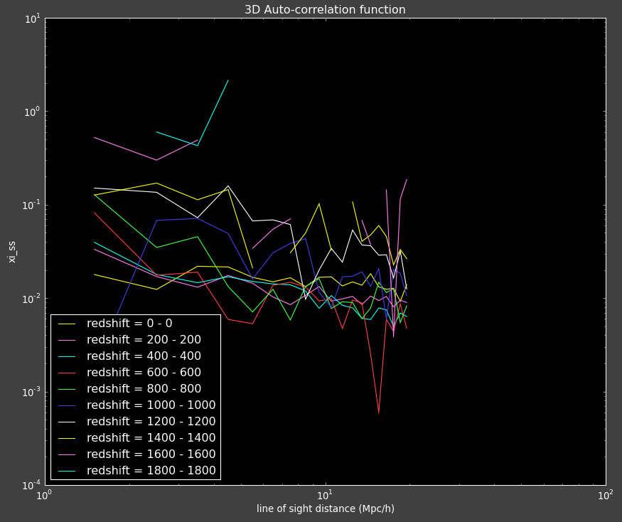
3D correlation functions for redshift bins

As you can see the 3D correlation function are no longer fluctuating around zero as they were on the Sloan data.

The reconstruction is a bit puzzling. Below is a histogram of the comoving distances (from the center of the sphere) of the spectroscopic (yellow), photometric (green) data sets as well as the reconstructed phi (redshift distribution (pink)). You will noticed that while the histograms don't match, the bumps in the photometric/spectroscopic histograms seem to match the bumps in phi. I was thinking that because these photometric/spectroscopic histograms include both the geometry and the "selection function" so to speak (I didn't actually apply a selection function, so it is just the natural clustering of the objects). Whereas phi (I think) is only supposed to be the selection function, not the geometry. I was wondering if perhaps if I subtract the geometry from the p/s histograms (which is proportional to r^2) then we would basically be left with these same wiggles? I've asked Alexia about this and I am waiting for a response.

Degrees vs. Radians

Turns out the "List length exceeded MaxList" error was due to the randoms not falling in the same region as the data. I had forgotten to convert my data from radians to degrees in Python (but it was being converted in the C program) and so the C-converted randoms (in x, y, z) did not match the Python-converted data (in x, y, z).

I've fixed this, and get the following 3D correlation functions for my redshift slices of the Mock data (and they look pretty darn good)!

My 3D Correlation function on Mock Data

This makes me want to make the bold statement that all the problems I was having with my 3D correlation functions on the Sloan data was a problem with the data, (not my code)... but I need to check this again because the 2D correlation functions looked ok on the Sloan data. This could be an issue of the photo-z's just being completely wrong, (David keeps saying he doesn't trust the CAS) so the 2D correlation function (which only uses ra and dec) is fine, but once we start using the photo-z's things get messed up.

Another thought I had was that I need to fix this declination random cosine population issue in the 2D correlation function, currently the declinations are being populated using a flat distribution.

Oh today is a good day indeed!

Correlation Correlation

Here are the angular cross correlation between the photometric data set and the binned spectroscopic data sets (12 -- one for each bin):

I also calculate the 3D auto-correlation function of spectroscopic data with itself (12 -- one for each bin):

The 3D correlation functions don't look very good to me. I would expect them to have a similar shape to the 2D correlation function, but I actually had to plot these on a normal plot (not log-log) because they were going negative. Alexia -- what do these look like for you on the mock data? I guess I should calculate them on the mock data myself.

Next step, reconstruction...

A Time to Reconstruct

Time for the moment of truth (again). I am confident that the 3D-correlation function is working properly and now I need to see if with these fixes the reconstruction work better.

Here is what I am doing:

I have a set of ~5 million Sloan galaxies from the CAS database. I take these galaxies and confine them to be in Stripe 82 ( -1.25< dec < 1.25 & 0 < ra < 120):

The data is confined to be in Stripe 82

I designate 20% of the 10^6 galaxies as the spectroscopic data set. The rest are my photometric data set. I convert the ra/dec/redshift to x/y/z (in comoving coordinates).

The data in both coordinate systems

I then bin the "spectroscopic" data into "redshift" bins. Below shows an example of one redshift bin (cyan) in the different coordinate systems:

For this run there were 12 bins, 200 Mpc/h wide, from 0 to 2400 Mpc/h.

Now to re-run my fixed correlation functions on the Sloan data, this take a day or so... Results to follow....