Going back to Working Reconstruction

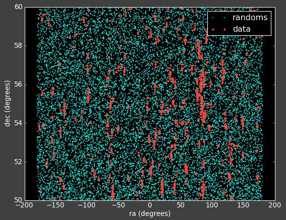
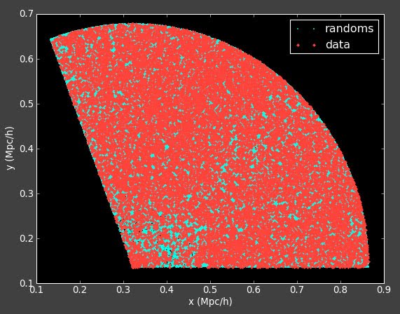
I spent today trying to reproduce the result from this post when the reconstruction was working on the Mock Data.

I got it working... here is the code (also in ../logs/110509log.py):

#~~~~~~~~~~~~~~~~~

import numpy as N

from pylab import *

from matplotlib import *

import crlold as crl

from correlationData import *

import galsphere as gals

import datetime as dt

workingDir = 'run2010211_1354'

# Create file names

mockLRGfile,photofile,specfile,corr2dfile,corr3dfile,photo2dfile,photoCDfile,spec2dfile,\

spec3dfile,argumentFile,runConstantsFile,wpsMatrixFile,xiMatrixFile=makeFileNames(workingDir)

oversample = 5.

corrBins = 40.0 #should be one more than you want it to be

mincorr = 0.01

maxcorr = 20.0

convo = 180./pi

corrspace = (maxcorr - mincorr)/corrBins

corrarray = makecorrarray(mincorr, maxcorr, corrspace)

nbins = 40

boxside = 1000.0 #in Mpc/h

xicorrmin = 0.001

xicorrmax = 20.0

nxicorr = 40

#make redshift bins

#boxside = 1000.0 #in Mpc/h

rbinmin = 0 #in Mpc/h

rbinspace = boxside/40 #in Mpc/h

rbinmax = boxside/2.0 + 0.0001 #in Mpc/h

rbins = makeRbins(rbinmin,rbinmax,rbinspace)

nrbins = rbins.size - 1

photoCD = readPhotoCDfile(photoCDfile)

#Create a matrix to input the correlation function data

# Write wps Matrix to file

#The number of redshift bins you want to skip for the

#reconstruction (this removes noisy bins from calculation)

skip = 0

makeWPSmatrix2(workingDir,rbins,corrBins, wpsMatrixFile, skip)

#Create a matrix to input the correlation function data

# Write Xi Matrix to file

makeXimatrix2(workingDir,rbins,nxicorr,xiMatrixFile, skip)

#Plot wps correlation functions

numtoplot = int(nrbins-skip) #number of correlation functions you want to display on plot

numtoplot = 10

plotWPSScreen(skip, numtoplot, workingDir, rbins)

pylab.legend(loc=1)

#Plot xi correlation functions

plotXiScreen(skip, numtoplot, workingDir, rbins)

# compute the xi matrix using the spec sample,

npbins=40#the number of bins you want reconstructed

reconstructmax = 0.5 #in Gpc

reconstructionmin = 0.0 #in Gpc

phibins = linspace(start=reconstructionmin,stop=reconstructmax,num=npbins,endpoint=True)

#phibins =(linspace(2,npbins,num=npbins,endpoint=False)+0.5)*(1./npbins)

sximat=crl.getximat(th,rlos,phibins,rs,xispec,xierr)

# invert to recover phi

phircvd=crl.getCoeff(wps,covar,sximat)

for i in range(len(phircvd.x)):

if (phircvd.x[i] < 0):

phircvd.x[i]=0

print 'the recovered selection function is not normalized.'

outphi4 = phircvd.x

phibins4 = phibins

start = 1

end = npbins - 1

#junkbins = linspace(start=0,stop=0.5,num=100,endpoint=True)

junkbins = phibins

junk = histogram(photoCD/1000., bins=junkbins)

junkdata = junk[0]

plot(junkbins[start:end], junkdata[start:end], 'r.-', label = 'photometric data')

plot((phibins4[start:end]+1.0*phibsize), outphi4[start:end]*sum(junkdata[start:end])/sum(outphi4[start:end]), 'g-', label = 'phi')

plot(phibins4[start:end],outphi4[start:end]*sum(junkdata[start:end])/sum(outphi4[start:end]),'c.-',label='reconstruction %i'%npbins)

#plot((phibins4[2:]-1.5*phibsize)/1000, phi[2:]*size(photoCD), 'g-', label = 'phi')

xlabel('comoving distance (Gpc/h)')

ylabel('number of objects per bin')

title('Redshift Distribution')

from pylab import *

legend(loc=2)

#~~~~~~~~~~~~~~~~~

It involved reverting back to an old version of crl (I saved it as crlold.py) and an older version of the plotting.

Here are the correlation functions:

I am getting the same problems with slight changes to the binning, changing how well the reconstruction works. For instance the best reconstruction is here (with 40 bins):

But if I change to 39 or 41 bins, I get a very different reconstruction:

Which makes me wonder if was just dumb luck that it worked for that particular binning in the first place.

I'm also running with a more interesting photometric distribution function to see how that looks. More to come....

Mask Fixed

It turns out that my mask was messing up. I now have it fixed. Here is what the data/randoms look like on the mock data:

And here is what is looks like for real data:

The log on 3/29 has the code to run these.

Playing with crl

I'm trying to fix the binning issues I was having with the reconstruction. Alexia suggested playing with the crl file.

In her email on March 10, subject: improving cross-correlation, she says:
"Go to the part of getCoeff in the crl.py file. There are two choices for for the matrix B (for a flat prior and for a linear prior). Comment out the linear and uncomment the flat, and rerun to see if you get the same behavior for a particular binning choice, or if you get the same TYPE of behavior with the new B, but not correlated to the specific bin choice."

I did above and here are some plots (left is with a constant prior and right is with linear prior):

This doesn't seem to change things much. I talked to Alexia on the phone today and she also suggested I change the value of lambda to see how that effects things.

Currently:
if tol > 0
lam*=10
else:
lam/=10

I'm looking at what changing these numbers (lambda) does to the reconstruction...

if lambda is 5:

Flat prior

Linear prior

if lambda is 100:
Flat prior

Linear Prior:

if lambda is 1:
Linear prior

Flat prior

Alexia doesn't think I should worry to much about this right now, but I thought I'd make some plots for her to look and think about.

On the to do list:
Run reconstruction on real data
Check the mesh to see if this is the cause of the correlation function taking so long to compute.

Back on Track

I fixed the angular correlation function using the method outlined in my last post. I did a run again on the mock data using photometric and spectroscopic sets with 200,000 objects. The correlation functions look much better now (and the code runs much faster too!):

2D and 3D correlation functions

The 2D are actual angular separations (different from what Alexia was doing which was collapsing the third dimension onto a projection plane). This is super exciting because the noise has gone down a lot compared to what I was getting before. Hopefully this will mean a better reconstruction.

The distribution functions I applied to the two data sets are below:

The cyan line is a histogram of the number photometric objects as a function of comoving distance away from the observer. The magenta line is the imposed photometric distribution function (what we are trying to reconstruct). The green line is a histogram of the number of spectroscopic objects as a function of comoving distance away from the observer. Note that it is different than the photometric distribution.

And here is the reconstruction:

The magenta is the imposed distribution function (same as the previous plot) and the red is the reconstructed distribution. They look pretty much the same. Awesome.

Back to Work (back to Reconstruction)

I need to do a better job of balancing working on both the Newman Project and BOSS Likelihood target selection. I feel like it's been months since I have worked on the Newman stuff. Luckily Alexia was in Mexico and helped me get up to speed again.

Martin White gave me a halo mock catalog (I was using the wrong one for a while) and I have applied the following selection function to the photometric data set:

This corresponds to the following redshift distribution (phi):

The blue line is a histogram of the redshifts of the mock data, and the green line is the phi we are imposing (by both geometry and the selection function, you can see they match pretty well). I believe the difference in these two is based on actual structure, not an problem with implementing the selection function.

On the spectroscopic data, I imposed no selection function, and so the distribution was based purely on the geometry and structure of the data. Because the geometry is a sphere, we expect more objects at greater redshifts (larger volume at greater r):

I decided to start with a small run with data sets of approximately equal size. The photometric data set has 25,887 objects, and the spectroscopic data set has 25,470 objects. The redshift bins are 50 Mpc/h wide and go from 0 - 500 Mpc/h. Here are the 2D cross-correlation functions and the 3D auto-correlation functions of the mock data:

Here is the reconstruction. It is using an old version of crl (I'm having trouble downloading the newest version from the repository). It doesn't seem to be doing that good of a job reconstructing:

Maybe updating crl will help things? Thoughts Alexia?

Mock Reconstruction

I ran a full reconstruction on the mock data over the past couple days. There are some problems with this run (which I discovered after I started it running, but decided to just let it finish). The first is that I have not fixed the distribution of the randoms in the 2D correlation function to go as cosine for the declinations (they are flat). The second is that I discovered the mock catalog I was using was not dark matter halos but actually LRGs and to the clustering properties are nonsensical. I have since gotten a dark matter halo catalog from Martin White.

Here are the 2D and 3D correlation function for the various redshift bins:

2D correlation functions for redshift bins


3D correlation functions for redshift bins

As you can see the 3D correlation function are no longer fluctuating around zero as they were on the Sloan data.

The reconstruction is a bit puzzling. Below is a histogram of the comoving distances (from the center of the sphere) of the spectroscopic (yellow), photometric (green) data sets as well as the reconstructed phi (redshift distribution (pink)). You will noticed that while the histograms don't match, the bumps in the photometric/spectroscopic histograms seem to match the bumps in phi. I was thinking that because these photometric/spectroscopic histograms include both the geometry and the "selection function" so to speak (I didn't actually apply a selection function, so it is just the natural clustering of the objects). Whereas phi (I think) is only supposed to be the selection function, not the geometry. I was wondering if perhaps if I subtract the geometry from the p/s histograms (which is proportional to r^2) then we would basically be left with these same wiggles? I've asked Alexia about this and I am waiting for a response.

Catalog Woes

It turns out my mock catalog is probably not what I want to be using. I talked to Alexia and Martin White, and I am using a LRG catalog, but I want to be using a halo catalog. This probably means that my clustering properties are nonsensical (because I am generating galaxies based on galaxies, not on halos). Martin said he is going to give me a better catalog to use.

In the mean time I am running on the catalog I have. The reconstruction should work as long as both the photometric and spectroscopic data sets are generated in the same way... even if they don't accurately represent any real distribution on the sky.

The reconstruction is currently running, and I should have it done later today.

I also checked my 3D slice against Alexia's to make sure they match, and they do:

My and Alexia's 3D Correlation functions on
a redshift slice of the mock data

Running Scripts (Update)

I want to utilize the fact that I can run the correlation function on multiple nodes of riemann. Eric helped me learn to use qsub to run a script on multiple nodes. I've got it working as follows:

In the file on riemann 091118jess.script there is the following:

#PBS -l nodes=1
#PBS -N jessjob1
#PBS -j oe
#PBS -M kirkpatrick@berkeley.edu
#PBS -V
cd /home/jessica/repository/ccpzcalib/Jessica/pythonJess
./runcode.script


where runcode.script contains the following:
python runReconstructionMock.py

I make both runcode.script and 091118jess.script executables, and then type in the terminal:
qsub 091118jess.script

I then exit from riemann/insure (didn't close it using x button, not sure if this makes a difference).

When I log back in the code is still running. (check using qstat)

Now I need to integrate this into the python code so that qsubs are generated for each correlation function for each redshift slice. This should make things go a lot faster.

The email from Eric:
----------
From: Eric Huff
Date: Wed, Nov 18, 2009 at 3:06 PM
Subject: qsub
To: Jessica Kirkpatrick

Here's a script example:

#PBS -l nodes=1
#PBS -l walltime=24:00:00
#PBS -m bea
#PBS -M emhuff@berkeley.edu
#PBS -V
ulimit -s unlimited
export PHOTO_DATA=/clusterfs/riemann/raid006/bosswork/groups/boss/photo/data
export PHOTO_REDUX=/clusterfs/riemann/raid006/bosswork/groups/boss/photo/redux
cd /home/emhuff/Coadds/Code/Coadd_Data_Root/Scripts
echo `hostname`
/home/emhuff/Coadds/Code/Coadd_Data_Root/Scripts/r.out 380720 6 0 00

And here's some online documentation for qsub:

http://www.doesciencegrid.org/public/pbs/qsub.html
http://njal.physics.sunysb.edu/tutorial-1.html

I'm running the full reconstruction on the mock data, I might have a fully working code tomorrow. Woo hoo!

Degrees vs. Radians

Turns out the "List length exceeded MaxList" error was due to the randoms not falling in the same region as the data. I had forgotten to convert my data from radians to degrees in Python (but it was being converted in the C program) and so the C-converted randoms (in x, y, z) did not match the Python-converted data (in x, y, z).

I've fixed this, and get the following 3D correlation functions for my redshift slices of the Mock data (and they look pretty darn good)!

My 3D Correlation function on Mock Data

This makes me want to make the bold statement that all the problems I was having with my 3D correlation functions on the Sloan data was a problem with the data, (not my code)... but I need to check this again because the 2D correlation functions looked ok on the Sloan data. This could be an issue of the photo-z's just being completely wrong, (David keeps saying he doesn't trust the CAS) so the 2D correlation function (which only uses ra and dec) is fine, but once we start using the photo-z's things get messed up.

Another thought I had was that I need to fix this declination random cosine population issue in the 2D correlation function, currently the declinations are being populated using a flat distribution.

Oh today is a good day indeed!

Exceeded Maxlist

I am getting a strange error when I run the 3D Correlation function. The error is from Martin White's meshing algorithm (nearmesh):

"List length exceeded MaxList=234700"

It think it happens when a point is near any mesh within the grid. But I am not sure exactly, I didn't write this section of the code, and I've never gotten this error before.

I wrote Alexia about it, and I am hoping she'll have some experience with this problem.

Below is the email I send her today:

-------
From: Jessica Ann Kirkpatrick
Date: Tue, Nov 17, 2009 at 11:24 PM
Subject: halo files and numbers
To: Alexia Schulz

Alexia,
the file I am using is from here: http://mwhite.berkeley.edu/Mock/

It was under a section that used to be there called LRG but now seems to be gone. See this blog entry.

The number of halos in the file is 102496.

When I run halolist with mmin = 5e10 I get 3811293 galaxies (for photometric data set)
When I run halolist with mmin = 5e11 I get 378932 galaxies (for spectroscopic data set)

output when I run halolist is below:

In [324]: #make galaxies
In [325]: mmin=5.e10 #for gal
In [326]: h=gals.halolist(mockLRGfile,mmin)
1.30144190788 seconds wall time to readin
1.3 seconds processor time to readin
33.0253970623 seconds wall time
30.84 seconds processor time

In [327]: g=gals.galist(h,nbins,outfile=photofile)
4.70264683703
halo number is 102496
number of halos with 1 or more gals 102496
176.569406033 seconds wall time
168.58 seconds processor time

In [328]: mmin=5.e11 #for spec
In [329]: h=gals.halolist(mockLRGfile,mmin)
10.7454509735 seconds wall time to readin
1.66 seconds processor time to readin
37.9757530689 seconds wall time
27.46 seconds processor time

In [330]: g=gals.galist(h,nbins,outfile=specfile)
4.70264683703
halo number is 102496
number of halos with 1 or more gals 101718
27.7532730103 seconds wall time
26.72 seconds processor time

I'm getting the error:
List length exceeded MaxList=234700
on one of my runs, has this ever happened to you?

It seems to be coming from deep in the calculation in the function meshnear.

I am getting this error when I try to run on redshift slices which are further away (and thus have higher statistics).

Tomorrow the BigBOSS meeting has a break from 12-1. Can I call you sometime in that window?
Cheers,
Jessica

--------

I thought perhaps a problem is that the randoms are not overlaping with the data (and so the nearmesh would mess up because the randoms are not in the same region as the data).

And this seems to be part of the problem:

Need to check these to see where the problem is. I think there might be a degrees vs radians issue. I'll look at this tomorrow.