Randoms for CFHT Galaxies

Spent the last couple days making the randoms for the CFHT galaxies. Here is how it's done:

; 1) Go to Analysis directory:

/home/jessica/repository/ccpzcalib/Jessica/qsobias/Analysis/

; 2) Make randoms for each pointing:

listfile = '/clusterfs/riemann/data/jessica/alexieData/se_cats/se_list.txt'

mask_dir='/clusterfs/riemann/data/jessica/alexieData/masks/'

infile = '/clusterfs/riemann/data/jessica/alexieData/Catalogs/cs82_all_cat1.fits'

random_dir = '/clusterfs/riemann/data/jessica/alexieData/randoms/'

make_randoms,infile,outfile,mask_dir,random_dir,listfile

; 3) Remove randoms not in mask, combine to single file

dir = '/clusterfs/riemann/data/jessica/alexieData/randoms/'

listfile = '/clusterfs/riemann/data/jessica/alexieData/se_cats/se_list.txt'

outfile = '/clusterfs/riemann/data/jessica/alexieData/Catalogs/random_catalog.fits'

fix_randoms,dir,listfile,outfile

; 4) Remove overlaping regions

infile = '/clusterfs/riemann/data/jessica/alexieData/Catalogs/random_catalog.fits'

outfile = '/clusterfs/riemann/data/jessica/alexieData/Catalogs/random_catalog_no_overlaps.fits'

ra_list = '/home/jessica/repository/ccpzcalib/Jessica/qsobias/Analysis/S82.ra_cuts'

se_list_file = '/clusterfs/riemann/data/jessica/alexieData/se_cats/se_list.txt'

remove_overlaps,infile,outfile,se_list_file,ra_list

Here are some plots from DS9, blue circles are randoms that are kept, and red circles are randoms that are masked out. The green and yellow regions are masked regions:

The randoms are made at a density of 7.5*10D^5 per square degree. This is approximately 10X the density of the data.

Masked BOSS and SDSS Data

Here are my photometric and spectroscopic data sets, masked so that they have the same footprint in the sky:

Whole Footprint (photometric)

Red = Data, Green = Randoms

Up-close patch (photometric)

Red = Data, Green = Randoms

Whole Footprint (spectroscopic)

Magenta = Data, Cyan = Randoms

Up-close patch (spectroscopic)

Magenta = Data, Cyan = Randoms

Whole Footprint (both)

Spectroscopic: Magenta = Data, Cyan = Randoms

Photometric: Red = Data, Green = Randoms

Up-close patch (both)

Spectroscopic: Magenta = Data, Cyan = Randoms

Photometric: Red = Data, Green = Randoms

Distribution of Dec (spectroscopic)

Magenta = Data, Cyan = Randoms

Distribution of Dec (photometric)

Red= Data, Green = Randoms

Distribution of Dec (both)

Spectroscopic: Magenta = Data, Cyan = Randoms

Photometric: Red = Data, Green = Randoms

Distribution of RA (spectroscopic)

Magenta = Data, Cyan = Random

Distribution of Dec (photometric)

Red= Data, Green = Randoms

Distribution of RA (both)

Spectroscopic: Magenta = Data, Cyan = Randoms

Photometric: Red = Data, Green = Randoms

Distribution of Redshift (z) (spectroscopic)

Magenta = Data, Cyan = Randoms

Distribution of Redshift (z)

Red = spectroscopic redshifts, Magenta = photometric photo-z's

About BOSS Data from Percival

Got word from Will Percival over the weekend:
He said the mask for the data/randoms is here:

https://trac.sdss3.org/browser/repo/boss/bosslss/trunk/geometry/current_boss_geometry.ply

He said:
I used the current_boss_geometry, choosing sectors with > 70% completeness. I don't have this separately in a file I'm afraid, but you could easily create it by placing the random catalog within the current_boss_geometry file - taking the quoted numbers as the completeness.

I said:
Thanks for the response. In terms of the 'current_boss_geometry' file. Is this as old as the randoms/galaxy files? Because I could imagine a scenario where the geometry file covers MORE area than the data files (because more of the sky has been observed) and then when I apply this "mask" to my other data it would let in regions of the sky which are not in the BOSS data files.

He said:
The current_boss_geometry file will always cover a larger area than that of the galaxies observed with completeness > 70%. But you can only use those polygons that contain one of the randoms. This will cut it back.

I said:
Also, how are you dealing with the spectroscopic completeness when generating the randoms? Are you basically filtering for each sky polygon based on the completeness in the current_boss_geometry file? For instance if a polygon has 80% completeness, then only 80% of randoms generated in that polygon are kept?

He said:
Yes, this is what I'm doing, based on the number of observed galaxies over the number of targets.

Using the BOSS Randoms

I downloaded the latest BOSS data and randoms from Will Percival as Martin White suggested in my email exchange with him yesterday.

There are in the following location on the wiki:
https://trac.sdss3.org/wiki/BOSS/clustering/cats

I put them here on riemann:

/clusterfs/riemann/raid001/jessica/boss/
galaxy-wjp-main008-LOWZ-020211-cut.txt
random-wjp-main008-LOWZ-020211-cut-small.txt
galaxy-wjp-merge-CMASS-020211-cut.txt
random-wjp-merge-CMASS-020211-cut-small.txt

The format of these files is:
ra / degrees
dec / degrees
redshift
galaxy weight
sector completeness
close pair flag
THING_ID
MASK POLY ID
ID for galaxy in spAll file (not in std format)

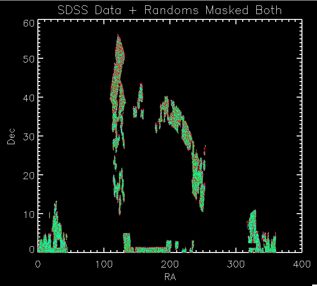
I read them in and below are plots. As you can see, the distribution of the randoms matches the data. So there is something wrong with what I am doing. At this point though, I'm not going to waste more time trying to fix my masks/randoms. I'm going to use these catalogs and re-run the correlation functions to see if this fixes things.

I'm also going to ask Shirley or Eric to run a correlation function on the same data to check that we get the same answer.



The code to make the above plots is in the following log file:
../logs/110302log/pro


thisfile = '/clusterfs/riemann/raid001/jessica/boss/galaxy-wjp-main008-LOWZ-020211-cut.txt'
readcol,thisfile,slra,sldec,slz,x,x,x,x,x,x,format='(F,F,F,F,F,F,F,F,F)'

thisfile = '/clusterfs/riemann/raid001/jessica/boss/galaxy-wjp-merge-CMASS-020211-cut.txt'
readcol,thisfile,sra,sdec,sz,x,x,x,x,x,x,format='(F,F,F,F,F,F,F,F,F)'

sra = [sra,slra]
sdec = [sdec,sldec]
sz = [sz,slz]



thisfile = '/clusterfs/riemann/raid001/jessica/boss/random-wjp-main008-LOWZ-020211-cut-small.txt'
readcol,thisfile,rslra,rsldec,rslz,x,x,x,x,x,x,format='(F,F,F,F,F,F,F,F,F)'

thisfile = '/clusterfs/riemann/raid001/jessica/boss/random-wjp-merge-CMASS-020211-cut-small.txt'
readcol,thisfile,rsra,rsdec,rsz,x,x,x,x,x,x,format='(F,F,F,F,F,F,F,F,F)'

rsra = [rsra,rslra]
rsdec = [rsdec,rsldec]
rsz = [rsz,rslz]



xtit = 'Ra'
ytit = 'Dec'
mtit = 'Ra vs Dec'
window,xsize=700,ysize=600
plot, sra, sdec, ps = 3, xrange = [110,130], yrange=[40,55],XTITLE = xtit, YTITLE =ytit, TITLE = mtit, charsize = 1.5, charthick = 1
oplot, rsra, rsdec, ps=3, color = fsc_color('green')



;Make histogram of the dec distributions
data = sdec
datamin = min(sdec)
datamax = max(sdec)
binsize = (datamax - datamin)/100
xtit = 'Dec Distribution'
ytit = '% in bin'
mtit = 'Histogram of Spectroscopic Dec'

window,xsize=700,ysize=600
hist = HISTOGRAM(data, binsize = binsize, min = datamin, max = datamax)
bins = FINDGEN(N_ELEMENTS(hist))*binsize + datamin
plot, bins, hist*1.0/n_elements(data), PSYM = 10, xrange = [datamin,datamax], yrange=[0,1.0*max(hist)/n_elements(data)],XTITLE = xtit, YTITLE =ytit, TITLE = mtit, charsize = 1.5, charthick = 1

data = rsdec
datamin = min(rsdec)
datamax = max(rsdec)
hist = HISTOGRAM(data, binsize = binsize, min = datamin, max = datamax)
bins = FINDGEN(N_ELEMENTS(hist))*binsize + datamin
oplot, bins, 1.0*hist/n_elements(data), PSYM = 10, color = fsc_color('green')



;Make histogram of the dec distributions
data = sdec
datamin = min(sdec)
datamax = max(sdec)
binsize = (datamax - datamin)/1000
xtit = 'Dec Distribution'
ytit = '# in bin'
mtit = 'Histogram of Spectroscopic Dec'

window,xsize=700,ysize=600
hist = HISTOGRAM(data, binsize = binsize, min = datamin, max = datamax)
bins = FINDGEN(N_ELEMENTS(hist))*binsize + datamin
plot, bins, hist*1.0, PSYM = 10, xrange = [datamin,datamax], yrange=[0,1.0*max(hist)],XTITLE = xtit, YTITLE =ytit, TITLE = mtit, charsize = 1.5, charthick = 1

data = rsdec
datamin = min(rsdec)
datamax = max(rsdec)
hist = HISTOGRAM(data, binsize = binsize, min = datamin, max = datamax)
bins = FINDGEN(N_ELEMENTS(hist))*binsize + datamin
oplot, bins, 1.0*hist, PSYM = 10, color = fsc_color('green')




;Make histogram of the dec distributions
data = sra
datamin = min(sra)
datamax = max(sra)
binsize = (datamax - datamin)/100
xtit = 'Ra Distribution'
ytit = '% in bin'
mtit = 'Histogram of Spectroscopic Ra'

window,xsize=700,ysize=600
hist = HISTOGRAM(data, binsize = binsize, min = datamin, max = datamax)
bins = FINDGEN(N_ELEMENTS(hist))*binsize + datamin
plot, bins, hist*1.0/n_elements(data), PSYM = 10, xrange = [datamin,datamax], yrange=[0,1.0*max(hist)/n_elements(data)],XTITLE = xtit, YTITLE =ytit, TITLE = mtit, charsize = 1.5, charthick = 1

data = rsra
datamin = min(rsra)
datamax = max(rsra)
hist = HISTOGRAM(data, binsize = binsize, min = datamin, max = datamax)
bins = FINDGEN(N_ELEMENTS(hist))*binsize + datamin
oplot, bins, 1.0*hist/n_elements(data), PSYM = 10, color = fsc_color('green')



;Make histogram of the dec distributions
data = sra
datamin = min(sra)
datamax = max(sra)
binsize = (datamax - datamin)/1000
xtit = 'RA Distribution'
ytit = '# in bin'
mtit = 'Histogram of Spectroscopic RA'

window,xsize=700,ysize=600
hist = HISTOGRAM(data, binsize = binsize, min = datamin, max = datamax)
bins = FINDGEN(N_ELEMENTS(hist))*binsize + datamin
plot, bins, hist*1.0, PSYM = 10, xrange = [datamin,datamax], yrange=[0,1.0*max(hist)],XTITLE = xtit, YTITLE =ytit, TITLE = mtit, charsize = 1.5, charthick = 1

data = rsra
datamin = min(rsra)
datamax = max(rsra)
hist = HISTOGRAM(data, binsize = binsize, min = datamin, max = datamax)
bins = FINDGEN(N_ELEMENTS(hist))*binsize + datamin
oplot, bins, 1.0*hist, PSYM = 10, color = fsc_color('green')



;Make histogram of the z distributions
data = sz
datamin = min(sz)
datamax = max(sz)
binsize = (datamax - datamin)/50
xtit = 'Redshift Distribution'
ytit = '% in bin'
mtit = 'Histogram of Spectroscopic z'

window,xsize=700,ysize=600
hist = HISTOGRAM(data, binsize = binsize, min = datamin, max = datamax)
bins = FINDGEN(N_ELEMENTS(hist))*binsize + datamin
plot, bins, hist*1.0/n_elements(data), PSYM = 10, xrange = [datamin,datamax], yrange=[0,1.0*max(hist)/n_elements(data)],XTITLE = xtit, YTITLE =ytit, TITLE = mtit, charsize = 1.5, charthick = 1

data = rsz
datamin = min(rsz)
datamax = max(rsz)
hist = HISTOGRAM(data, binsize = binsize, min = datamin, max = datamax)
bins = FINDGEN(N_ELEMENTS(hist))*binsize + datamin
oplot, bins, 1.0*hist/n_elements(data), PSYM = 10, color = fsc_color('green')



;Plot Data that is inside the mask
window,xsize=700,ysize=600
xobject = sra
yobject = sdec
xtit = 'RA'
ytit = 'Dec'
mtit = 'SDSS Spectroscopic Data + Masks'
plot, xobject, yobject, psym=3, symsize=2, XTITLE = xtit, YTITLE = ytit, TITLE = mtit, charsize = 2, charthick = 1, thick = 2, xthick=2, ythick=2
oplot, xobject, yobject, ps=3, color=fsc_color('white')
oplot, rsra, rsdec, ps=3, color=fsc_color('green')

Mask Help From Martin White

Hi Jessica,

I don't remember exactly what I did to make the mask you're using, but those plots look more or less right, I'm not sure what you were keying on? In addition to dropping regions below 75% completeness I also threw away regions whose area was too small to reliably estimate a completeness -- that leads to small "gaps" in the mask. And the mask was made on the plates observed up until June (I think) last year and only included the higher z (CMASS) sample. Which part of the zoom in plot is worrying you? I assume that's the one you're worried about?

Of course, those files are very out of date now compared to the current situation and should probably be redone -- quite a lot has changed since then.

Martin.

~~~~~~~~
Martin,
The actual concern stems from the fact that the ra/dec distribution of the randoms I generate using this mask, do not match (within expected noise) to the distribution of the data. This caused me to wonder if perhaps I am applying the mask incorrectly. This is my first time working with mangle.

Here are plots of the masked data and masked randoms along with the distribution histograms. Note that both of these data sets have the same number of objects: 139874. In these plots the masked BOSS data is white and the masked randoms are green.

You'll notice that there are ra/dec regions where there are over densities of the randoms or the data much more than what you would expect due to Poisson noise. I've shown this by binning both roughly (50 bins) and finely (1000 bins). In the fine binning you can see what the noise levels are.








The way I am generating these randoms is as follows (code is at bottom of email):
1) Read in the BOSS Mask
2) Generate a set of random ra and dec values
3) Check if random ra/dec is in the mask
4) Cut set of randoms to only be items in side the mask
5) Get the polygon weight for each random in the mask
6) Generate a random "test weight" a value between 0 and 1 for each random.
7) If the "test weight" is less than or equal to the polygon weight for that random, keep the random.
8) Otherwise throw out the random. This assures that the completeness of the randoms matches that of the BOSS data.
9) Repeat above process until you get the desired number of randoms

I've talked to both David and Shirley about this and they seem to think this is the correct way to generate the randoms. So I am confused as to why the distributions don't match. I would think the clustering of the BOSS data would be on a smaller order than the bin sizes of the attached histograms.

Any insight you have on this problem would be wonderful.

Also, it would be useful to have a mask for the current BOSS data set, as you said the one I have is quite out of date. Is this mask continuously generated? Where could I download it? Or do you need to do it manually?

Thank you again for any ideas you have.
Jessica


Here is the code to generate the randoms:
; Read in BOSS Mask

bossmask = "/clusterfs/riemann/raid001/jessica/boss/bossX.002.ply"
read_mangle_polygons, bossmask, polygons, id

;Ignore mangle polygons where the pixel weight is zero
bosspolygons = polygons[where(polygons.weight GT 0)]

;Generate a set of random ra/dec:
randomdec = 90.0-acos(RANDOMU(S, 10*randomsize)*2.0-1.0)*180./!

p
randomra = RANDOMU(S, 10*randomsize)*360.

;Select objects in mask
results = is_in_window(ra=randomra,dec=randomdec,bosspolygons,in_polygon=polynum)
inBossMask = where(results EQ 1)
polys = polynum[inBossMask]

;Get weights of the randoms
randomweights = bosspolygons[polys].weight

;Cut the Ra/Dec such that it is in the BOSS Mask
rsra = randomra[inBossMask]
rsdec = randomdec[inBossMask]

; Keep or throw out a random based on the weight of the pixel it is generated in:
; Assign a random test weight, only keep randoms whose test weight
; is less than or equal to the weight of that pixel (randomweights).
; So if the weight of a pixel is 0.8 then 80% of randoms generated in that pixel will be kept.
weighttest = RANDOMU(S, n_elements(randomweights))
isobserved = where(weighttest LE randomweights)

;Randoms inside mask, weighted properly
randomra = rsra[isobserved]
randomdec = rsdec[isobserved]

thisra = randomra
thisdec = randomdec

(repeat until get the desired number of randoms)

----------

Jessica,

Ok, I'm not sure that I understand that and I don't know much (i.e. anything) about the IDL versions of Mangle routines. We can try a few spot tests quickly though. First, a more up-to-date mask. I don't have the latest mask (Will has taken over generating those) but I have one that's fairly close. I put it on Riemann in the BOSS subdirectory of my home directory:

/home/mwhite/BOSS/bossX.004.

ply

For that file I just generated a bunch of random points and asked what the polygon ID and weights were. See if your code agrees with this:

# RA DEC PolyID Weight
120.22085116 44.18548740 2395 0.8810
115.07126735 41.20294362 2276 0.0000
111.08122943 41.50788940 2458 0.9365
122.77802060 40.69059229 2520 0.9615
120.27949275 40.36484626 2501 0.8905
110.35797556 40.43283558 2453 0.0000
125.63829796 40.93875235 2542 0.9833
117.66991611 40.36353309 2324 0.7857
112.57187913 41.52219305 2452 0.9158
123.30608484 40.38555016 2522 0.9130

If you agree then I suspect everything is fine. If not, we can figure out what the differences are and try to fix them.

By the way ... there is a command ("ransack" I think) for generating random points which is part of the Mangle software package. And Will is supplying random catalogs now as part of his catalog efforts. They are available off the LSS pages on the BOSS Wiki.

Martin

-----

Martin,
Thank you for helping me debug this.

I get the same numbers as you below for polyID and weight. I guess I'll try using Will's random catalogs and see if that helps things.

I appreciate your time.
Jessica

----

Here is the code I used for the test:

testra = [120.22085116, 115.07126735, 111.08122943, 122.77802060, 120.27949275, 110.35797556, 125.63829796, 117.66991611, 112.57187913, 123.30608484]
testdec = [44.18548740, 41.20294362, 41.50788940, 40.69059229, 40.36484626, 40.43283558, 40.93875235, 40.36353309, 41.52219305, 40.38555016]
testpolyID = [2395, 2276, 2458, 2520, 2501, 2453, 2542, 2324, 2452, 2522]
testweight = [0.8810, 0.0000, 0.9365, 0.9615, 0.8905, 0.0000, 0.9833, 0.7857, 0.9158, 0.9130]

bossmask = "/clusterfs/riemann/raid001/jessica/boss/bossX.004.ply"
read_mangle_polygons, bossmask, polygons, id
results = is_in_window(ra=testra,dec=testdec,polygons,in_polygon=polynum)
weight = polygons[polynum].weight
polyID = id[polynum]

Making Randoms within Mask

I spent the weekend trying to make random catalogs inside the masks. They are taking forever to run, so I probably need to optimize better. I didn't spend too much time doing this before because I figured we would only need to make the random catalogs once and then we could just use them over and over again.

However, I've been running the code to generate them for > 13 hours and they still haven't finished, so there is a problem somewhere. The issue is that the mask represents a small region of the sky, but I am generating random objects over the whole sky, so 99.99% of the objects are rejected and thus the code is very inefficient.

Update: I found a bug in this code while trying to optimize explains why it was taking so long to run. Here is some testing about how it scales with number of randoms generated:

photo randoms:
500 randoms
Mon Dec 13 22:28:44 2010
Mon Dec 13 22:29:13 2010
29 seconds

5000 randoms
Mon Dec 13 22:34:00 2010
Mon Dec 13 22:31:02 2010
~3 minutes

50,000 randoms
Mon Dec 13 22:36:04 2010
Mon Dec 13 23:02:00 2010
~28 minutes

spectro randoms:
500 randoms
Mon Dec 13 22:32:10 2010
Mon Dec 13 22:31:45 2010
25 seconds

5000 randoms
Mon Dec 13 22:37:06 2010
Mon Dec 13 22:34:38 2010
~2.5 minutes

50,000 randoms
Mon Dec 13 22:38:51 2010
Mon Dec 13 23:01:42 2010
~23 minutes

The way the code works in it's current (inefficient) form:

For Spectroscopic Data:
1) Read in the two masks.
2) Create random ra and dec that are 5X as big as the spectro data set
3) Assign a redshift from the redshifts of the spectro data set (to keep same redshift distribution)
4) See if ra/dec is in the both masks
5) If it is in both masks, look at the weight in the BOSS mask. Assign a random weight to the object (between 0 and 1), if it is less than or equal to the weight of the BOSS mask then it is "observed", if it is greater than the BOSS weight it "isn't observed"
6) Repeat above until you reached the right number of randoms

For Photometric Data:
1) Read in the two masks.
2) Create random ra and dec that are 5X as big as the photo data set
3) See if ra/dec is in the both masks
4) Repeat above until you reached the right number of randoms

We don't need to assign a redshift to the photo data or "observe or not observe" because the photometric data doesn't have weights.

The code is here:

../pcode/photorandoms.pro
../pcode/spectrorandoms.pro

The code to run this as a qsub is here:
../pcode/makeRphoto.script
../pcode/makeRspec.script

You run it with the following code:
qsub makeR[photo,spec].script

The randoms have the same distribution as the data, shown in the following histograms, white is the data, red is the randoms:



Sweet!

At Los Alamos

I am visiting Alexia at Los Alamos National Lab for the next three weeks. Los Alamos is beautiful, but COLD.

I'm putting the final touches on the data-correlation function setup.

I noticed that in the 3D auto-correlation, I am producing two different random catalogs and using the following calculation:

(dd -dr1 -r2d +r1r2)/(r1r2)

This might be extra computing power than necessary if it is ok for r1 = r2... but I forget if they need to be different... perhaps they do need to be different in order for this to work. It seems like this is something I would have thought of before.

I talked to Alexia about this and she thinks it shouldn't make a difference either way. So I am going to set r1 = r2 and see what happens....

Old Autocorrelation Function results (without randoms fed in)
# r (Mpc/h) cross xi (r)
# r (Mpc/h) cross xi (r)
1.0009750000 113.0999999998
3.0009250000 4.3312368973
5.0008750000 0.1890557940
7.0008250000 0.3768587361
9.0007750000 0.4359240581
11.0007250000 0.1349752029
13.0006750000 0.1273595140
15.0006250000 -0.1351841518
17.0005750000 0.2378351539
19.0005250000 0.2994336370
21.0004750000 -0.0479553597
23.0004250000 -0.0998846930
25.0003750000 -0.1438266200
27.0003250000 -0.3070417433
29.0002750000 -0.3108741254
31.0002250000 -0.1177777522
33.0001750000 -0.0633376228
35.0001250000 -0.2604527820
37.0000750000 -0.2517495550
39.0000250000 -0.0304629134


New Autocorrelation Function results (with randoms fed in)
I think small differences are rounding errors
# Reached checkpoint 4
# r (Mpc/h) cross xi (r)
1.0009750000 113.0999999998
3.0009250000 4.3294918806
5.0008750000 0.1890963726
7.0008250000 0.3766263941
9.0007750000 0.4359240581
11.0007250000 0.1349752029
13.0006750000 0.1273650408
15.0006250000 -0.1355281973
17.0005750000 0.2380827199
19.0005250000 0.2995001354
21.0004750000 -0.0479749624
23.0004250000 -0.0998864926
25.0003750000 -0.1437953465
27.0003250000 -0.3070974753
29.0002750000 -0.3107744869
31.0002250000 -0.1177689518
33.0001750000 -0.0632545877
35.0001250000 -0.2605975485
37.0000750000 -0.2517029624
39.0000250000 -0.0304363094

New Autocorrelation Function with r1 = r2 (with randoms fed in)
There are pretty big difference between these two, but this could just be because my data set is small. Should check on a larger set.
# Reached checkpoint 4
# r (Mpc/h) cross xi (r)
1.0009750000 120.9999999998
3.0009250000 3.9579487179
5.0008750000 0.1234024722
7.0008250000 0.3826803206
9.0007750000 0.4731333382
11.0007250000 0.0871628790
13.0006750000 0.0808080808
15.0006250000 -0.1168749344
17.0005750000 0.2334021835
19.0005250000 0.3148748159
21.0004750000 -0.0339674194
23.0004250000 -0.0762365727
25.0003750000 -0.1365716955
27.0003250000 -0.2876355988
29.0002750000 -0.3209356312
31.0002250000 -0.1164599148
33.0001750000 -0.0517181534
35.0001250000 -0.2402264337
37.0000750000 -0.2732306595
39.0000250000 -0.0168706759

Masking both Data and Randoms

I've masked both the data and the randoms now:


The randoms (magenta) now fall exactly on top of the data (cyan). The code to do this is as follows:

;Read in data
file1 = "/home/shirleyho/research/SDSS_PK/powerspec_dir/DATA/ra_dec_z_run_rerun_camcol.z_gt_0.01"

readcol, file1, RA, DEC, z, RUN, rerun, camcol, x, x, x, x, x, x, x, x, format='(F,F,F,D,D,D,D,D,F,F,F,F,F,F)'

datasize = n_elements(ra)

;Read in mask
file = "/home/shirleyho/research/SDSS_PK/powerspec_dir/MASK_SDSS/dir_fits/tmp_unified_score_ebv_psf_bsm_nside1024.fits"

read_fits_map, file, weight, nside=nside_in, ordering=order


index = 0L
;Convert ra/dec to phi/theta expected in HEALPix
dataphi = ra*!pi/180.
datatheta = (90.0-dec)*!pi/180.
;Will be filled in with weight corresponding to ra/dec of data
dataweight = findgen(datasize)*0.0

;Function I wrote to get the weight for the data
junk = maskdata(datatheta, dataphi, index, datasize, nside_in, weight, dataweight)
;Only keeps data with a weight greater than 0.2 (inside mask)
datacut = where(dataweight GE 0.2)

;Make the randoms
randomsize = datasize*5L
randomtheta = findgen(randomsize)*0.0
randomphi = findgen(randomsize)*0.0
index = 0L
;Function I wrote to fill in randomtheta and randomphi with points inside the mask
junk = makemaskrandoms(randomtheta, randomphi, index, randomsize, nside_in, weight)

;Plot the data and the randoms
plot, ra[sub], dec[sub], psym=3, symsize=2, xr=[0,360],yr=[0,90], XTITLE = "RA", YTITLE = "DEC", TITLE = "RA vs Dec of Data and Randoms", charsize = 2, charthick = 1, thick = 2, xthick=2, ythick=2
oplot, ra[datacut], dec[datacut], psym=3, color=fsc_color('cyan')
oplot, randomra[0:100000], randomdec[0:100000], psy = 3, color=fsc_color('magenta')

Now to compute some correlation functions!

Plot of Data / Randoms

Here is a plot of the data (cyan) and randoms (magenta) using the masks, and the method outlined in this post:

I'm a little confused as to why some of the data isn't represented in the randoms. It seems the mask is different than the data, perhaps this is because there is less completeness in the regions that aren't covered in the mask. I'll ask Shirley about this, but in the mean time, I'll apply the mask to both the data and the randoms, to insure the area covered are the same.


11/2 Update: Heard back from Shirley she says:

"This is deliberate. And your plot reflects it :)

There is a reason to cut out certain areas in the mask, and I never said that the data covers the same area as the mask :) ! I am testing things right now for different areas to cut out :) ! (due to extinction, stars and possible photometric calibration problems)"

So I looks like I should just apply the mask to both the data and the randoms before doing the cross correlation, as I suspected.

Code for Random Catalog with Mask

From Wolfram Math World:

To pick a random point on the surface of a sphere, it is incorrect to select spherical coordinates θ and φ from uniform distributions θ ∈ [0,2π) and φ ∈ [0,π], since the area element dΩ=sinφdθdφ is a function of φ, and hence points picked in this way will be "bunched" near the poles (left figure above).

To obtain points such that any small area on the sphere is expected to contain the same number of points (right figure above), choose u and v to be random variates on (0,1). Then

θ = 2πu

φ = cos^-1(2v - 1)

gives the spherical coordinates for a set of points which are uniformly distributed over the surface of the sphere. This works since the differential element of solid angle is given by

dΩ = sinφdθdφ = -dθd(cosφ)

So for us to pick a random ra and dec on the sphere we want to use the following in idl:

theta = 2*!pi*RANDOMU(S, 1)
phi = acos(2*RANDOMU(S, 1) - 1)

This should give us a random theta and phi where θ ∈ [0,2π) and φ ∈ [0,π].

Unfortunately, just to be difficult HEALPix expects the following as inputs for ang2pix_nest:

theta - angle (along meridian), in [0,Pi], theta=0 : north pole
phi - angle (along parallel), in [0,2*Pi]

So their convention is the opposite of mine above so we should use the following:
phi = 2*!pi*RANDOMU(S, 1)
theta = acos(2*RANDOMU(S, 1) - 1)

Here is the code:

file = "maskfile.fits"
; nside_in is the number of pixels n the mask
read_fits_map, file, weight, nside=nside_in, ordering=order

; make random phi and theta
phi = 2*!pi*RANDOMU(S, 1)
theta = acos(2*RANDOMU(S, 1) - 1)

; Find pixel ipnest
ang2pix_nest, nside_in, theta, phi, ipnest

; Find weight of pixel
thisweight = weight[ipnest]

; check to make sure pixel center (thistheta, thisphi) is close to phi and theta
pix2ang_nest, nside_in, ipnest, thistheta, thisphi

(Checked this for several theta/phi and it looked good)


So here is the code to make the random catalog of size randomsize:

randomsize = 100
randomtheta = findgen(randomsize)*0.0
randomphi = findgen(randomsize)*0
index = 0

while index lt randomsize do begin
    thisindex = index 
    while index eq thisindex do begin
       phi = 2*!pi*RANDOMU(S, 1)
       theta = acos(2*RANDOMU(S, 1) - 1)
       ang2pix_nest, nside_in, theta, phi, ipnest
       thisweight = weight[ipnest]
       if thisweight gt 2.0 then begin
          randomtheta[index] = theta
          randomphi[index] = phi
          index = index+1
       endif  
    endwhile
endwhile

Another idea...

Another idea I have about generating this random catalog. First I generate the random ra and random dec, then I use the function ang2pix_nest (converts angle to pixel) to figure out which pixel it occurs in. Once we have that, depending on the weight we can keep the random value or throw it away. However, this might take a really long time if most of our objects are outside of the mask.

I also am not sure how to use the weight value. Should it be a step function, if weight > 0.2 then keep, if not then throw away, or something more subtle like the weight represents the expectation value of the probability distribution of if the random is in the pixel or not. In terms of the redshifts, should I do what I did before and match the random redshift distribution to the data?

Learning About HEALPix

I've been playing with Shirley's LRG catalog and mask. The mask uses something called HEALPix which I've never used before. It basically breaks up the spherical sky into equal area pixels:



The map is in the form of weights for each pixel. Shirley says that if the weight is greater than 0.2 she considers that pixel in the mask.

So to create a random catalog, I just go through the weights, and if it is greater than 0.2 I place objects in that pixel.

The key is to now convert from a Healpix mask to ra/dec.
There are two routines that do this that I have found:

DPF_PIX2ANG_NEST
pix2ang_nest

The problem is that these routines return the ra/dec of the center of the pixel. And to avoid putting extra power at the separations of the pixels, we want to select random points within the pixel. However, as you can see below, the ra range of these pixels changes dramatically as a function of cos (theta) (i.e. large at the poles and small at the equator) and so it isn't a simple procedure to fill in the area of a pixel evenly with random points:


I've searched to see if there is an existing package that does this, and I can't seem to find anything. In the HEALPix documentation there is a comment on random number generation, it doesn't seem to be what I am interested in here. I also have a email out to Shirley about this.

There are many functions that deal with HEALPix on their web page and well as in IDLUTILS. I'm currently combing through them to see if there is a function that gives me the ra/dec ranges for a given pixel, or even better, automatically picks a random point given a pixel.

Some questions:

1. How do I assign a random place in a HEALPix pixel and convert this to a ra/dec position?
2. The mask contains a "weight" for each HEALPix pixel, how to do factor in the weight into the random catalog. My intuition is that pixel's with higher weight should have more objects in them, but will this add clustering signal to the random catalog that we don't want?
   
3. How do we distinguish what is signal because of observation effects (we only looked at that patch of the sky once, or we didn't target as many objects there) and what is signal due to clustering of the data (there is a huge galaxy cluster in that part of the sky, and that is why there is more data there)?
   

Degrees vs. Radians

Turns out the "List length exceeded MaxList" error was due to the randoms not falling in the same region as the data. I had forgotten to convert my data from radians to degrees in Python (but it was being converted in the C program) and so the C-converted randoms (in x, y, z) did not match the Python-converted data (in x, y, z).

I've fixed this, and get the following 3D correlation functions for my redshift slices of the Mock data (and they look pretty darn good)!

My 3D Correlation function on Mock Data

This makes me want to make the bold statement that all the problems I was having with my 3D correlation functions on the Sloan data was a problem with the data, (not my code)... but I need to check this again because the 2D correlation functions looked ok on the Sloan data. This could be an issue of the photo-z's just being completely wrong, (David keeps saying he doesn't trust the CAS) so the 2D correlation function (which only uses ra and dec) is fine, but once we start using the photo-z's things get messed up.

Another thought I had was that I need to fix this declination random cosine population issue in the 2D correlation function, currently the declinations are being populated using a flat distribution.

Oh today is a good day indeed!

Exceeded Maxlist

I am getting a strange error when I run the 3D Correlation function. The error is from Martin White's meshing algorithm (nearmesh):

"List length exceeded MaxList=234700"

It think it happens when a point is near any mesh within the grid. But I am not sure exactly, I didn't write this section of the code, and I've never gotten this error before.

I wrote Alexia about it, and I am hoping she'll have some experience with this problem.

Below is the email I send her today:

-------
From: Jessica Ann Kirkpatrick
Date: Tue, Nov 17, 2009 at 11:24 PM
Subject: halo files and numbers
To: Alexia Schulz

Alexia,
the file I am using is from here: http://mwhite.berkeley.edu/Mock/

It was under a section that used to be there called LRG but now seems to be gone. See this blog entry.

The number of halos in the file is 102496.

When I run halolist with mmin = 5e10 I get 3811293 galaxies (for photometric data set)
When I run halolist with mmin = 5e11 I get 378932 galaxies (for spectroscopic data set)

output when I run halolist is below:

In [324]: #make galaxies
In [325]: mmin=5.e10 #for gal
In [326]: h=gals.halolist(mockLRGfile,mmin)
1.30144190788 seconds wall time to readin
1.3 seconds processor time to readin
33.0253970623 seconds wall time
30.84 seconds processor time

In [327]: g=gals.galist(h,nbins,outfile=photofile)
4.70264683703
halo number is 102496
number of halos with 1 or more gals 102496
176.569406033 seconds wall time
168.58 seconds processor time

In [328]: mmin=5.e11 #for spec
In [329]: h=gals.halolist(mockLRGfile,mmin)
10.7454509735 seconds wall time to readin
1.66 seconds processor time to readin
37.9757530689 seconds wall time
27.46 seconds processor time

In [330]: g=gals.galist(h,nbins,outfile=specfile)
4.70264683703
halo number is 102496
number of halos with 1 or more gals 101718
27.7532730103 seconds wall time
26.72 seconds processor time

I'm getting the error:
List length exceeded MaxList=234700
on one of my runs, has this ever happened to you?

It seems to be coming from deep in the calculation in the function meshnear.

I am getting this error when I try to run on redshift slices which are further away (and thus have higher statistics).

Tomorrow the BigBOSS meeting has a break from 12-1. Can I call you sometime in that window?
Cheers,
Jessica

--------

I thought perhaps a problem is that the randoms are not overlaping with the data (and so the nearmesh would mess up because the randoms are not in the same region as the data).

And this seems to be part of the problem:

Need to check these to see where the problem is. I think there might be a degrees vs radians issue. I'll look at this tomorrow.

Data Fixed?

I wanted to see if the changes I made to the declination distribution of the randoms fixed the problem with the Sloan data 3D correlation function. It appears it has not.

The correlation function is going negative ~5 Mpc/h:

As per Nic Ross's advice I am printing out the individual elements of the correlation function:

bin dd dr rd rr

0 317762.000000 216879.000004 217092.400004 226377.000004
1 1438272.000000 1190313.799866 1189213.999867 1244237.199854
2 2708480.000000 2477950.600010 2481026.000013 2551443.400078
3 3778250.000000 3627401.601080 3635341.801088 3668580.801119
4 4493904.000000 4437785.801835 4441650.801839 4424500.401823
5 4827204.000000 4858547.602227 4850951.402220 4790191.802163
6 4832844.000000 4926666.002291 4915620.202280 4845375.602215
7 4632790.000000 4742744.802119 4739360.602116 4702071.602081
8 4356652.000000 4461201.001857 4459481.601855 4483517.001878
9 4157056.000000 4233592.001645 4233477.601645 4276671.401685
10 4014424.000000 4070859.001493 4070540.001493 4105703.401526
11 3903134.000000 3944458.201376 3945670.001377 3970457.201400
12 3811114.000000 3847011.401285 3849257.601287 3867510.001304
13 3745984.000000 3769143.601212 3771384.201215 3788595.401231
14 3684692.000000 3707139.601155 3706282.401154 3723841.201170
15 3632222.000000 3651903.001103 3652026.201103 3667982.201118
16 3582504.000000 3600661.601056 3600676.801056 3617006.401071
17 3541194.000000 3554850.401013 3556219.601014 3567875.401025
18 3505996.000000 3511868.800973 3511927.400973 3523757.600984
19 3464186.000000 3468078.800932 3468489.800932 3482728.600946
20 3418956.000000 3425039.800892 3424701.000892 3442556.200908
21 3376304.000000 3386133.600856 3386409.600856 3406330.600875
22 3348124.000000 3351585.600824 3351850.400824 3371267.600842
23 3312086.000000 3319740.000794 3317782.400792 3335477.000809
24 3278338.000000 3285228.400762 3283852.800761 3299746.600775
25 3237588.000000 3252288.800731 3251628.800731 3266714.800745
26 3207848.000000 3220719.400702 3217525.800699 3234663.000715
27 3184346.000000 3189389.600673 3187092.600670 3199858.800682
28 3154432.000000 3160154.200645 3157859.200643 3168571.000653
29 3127406.000000 3131088.200618 3127228.000615 3137800.800625
30 3093844.000000 3098019.600587 3096805.400586 3105624.200595
31 3064538.000000 3064802.600557 3064300.800556 3072282.600563
32 3036138.000000 3035210.800529 3032522.400526 3040139.800534
33 2999470.000000 3000089.200496 3000837.800497 3008239.000504
34 2962448.000000 2968977.200467 2970271.600468 2979345.000477
35 2927012.000000 2934725.000435 2935492.800436 2946856.400447
36 2901310.000000 2903968.800407 2902961.000406 2913088.800415
37 2863636.000000 2869294.400374 2869514.600375 2881526.600386
38 2821798.000000 2833074.200341 2834320.800342 2847371.800354
39 2796586.000000 2803686.200313 2803161.600313 2813829.200323

Because the dr an rd are being subtracted from rr and dd in the calculation of the correlation function, it is possible for the correlation function to go negative if the objects are more correlated with the random data than with themselves. This seems very strange to me, but it is possible that because we don't trust the photo-z's from the data set I am using that maybe this is causing the problem?

I think the next step is to run the reconstruction purely on the mock data to see if that works, and this should isolate if this is a bad data issue or a bad code issue.

Populating the Sphere

I am trying to populate the randoms in the same way that the data is populated over the sphere. This means that in right ascension I populate the randoms with a uniform distribution over the range of the data values. However, for declination I populate using a cosine function (because we want to density per volume element to be constant). I am doing the following:

oo = 1;
while(oo){
   thisdec = drand48()*mask;  // Choose a declination inside the mask
   theta = drand48();  //Choose a random value for sin(thisdec)
   /*If theta is "below the sin(thisdec) curve",
   keep thisdec, otherwise repeat above process. */
   if(theta < sin(thisdec){
     Rb[nn].pos[i] = thisdec;
     oo = 0;
  }
}

This uses a rejection sampling method to populate the declinations. It seem to work, here are plots of the random distributions compared with the data, you can see that the distributions match:

Matching distributions of data (red) and randoms (blue)

Just to make sure that the data still falls in the same regions as the randoms here are more plots:

The data (red) falls in the same physical region as the randoms (blue)

Now my correlation function matches Alexia's again (as opposed to my October 30th post):

Matching 3D correlation functions!