More QSO-Galaxy Cross Correlations

Here are the QSO-Galaxy Cross-Correlations comparing high/low redshift QSOs. I divide the QSO sample in half (0.5 < z < 0.77) & (0.77 < z <1.0):

(plots on wiki)

Here are the QSO-Galaxy Cross Correlations comparing bright/dim QSOs. I divide the QSO sample into the 1/3 brightest (20.20 < g-mag < 16.17) and 1/3 dimest (25.87

(plots on wiki)

It's pretty interesting that there seems to be a difference in the correlation functions for bright/dim objects. I am not sure if we should expect this. The redshift distribution of these objects is similar, so that points to the fact that these objects are actually brighter (not sure further away). I'm hoping to do this in terms of high/low luminosity... but I need to figure out the absolute magnitudes of these objects first. Have pinged Ross about this. More to come...

Masked BOSS and SDSS Data

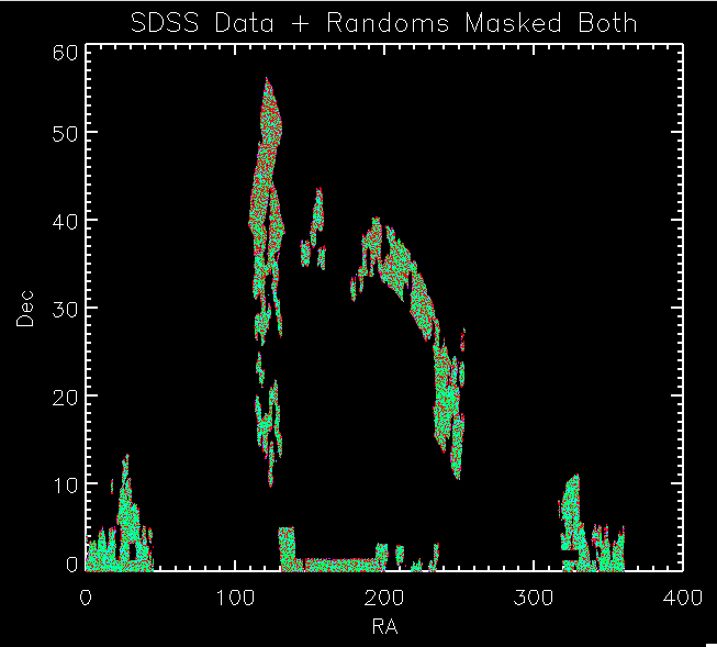
Here are my photometric and spectroscopic data sets, masked so that they have the same footprint in the sky:

Whole Footprint (photometric)

Red = Data, Green = Randoms

Up-close patch (photometric)

Red = Data, Green = Randoms

Whole Footprint (spectroscopic)

Magenta = Data, Cyan = Randoms

Up-close patch (spectroscopic)

Magenta = Data, Cyan = Randoms

Whole Footprint (both)

Spectroscopic: Magenta = Data, Cyan = Randoms

Photometric: Red = Data, Green = Randoms

Up-close patch (both)

Spectroscopic: Magenta = Data, Cyan = Randoms

Photometric: Red = Data, Green = Randoms

Distribution of Dec (spectroscopic)

Magenta = Data, Cyan = Randoms

Distribution of Dec (photometric)

Red= Data, Green = Randoms

Distribution of Dec (both)

Spectroscopic: Magenta = Data, Cyan = Randoms

Photometric: Red = Data, Green = Randoms

Distribution of RA (spectroscopic)

Magenta = Data, Cyan = Random

Distribution of Dec (photometric)

Red= Data, Green = Randoms

Distribution of RA (both)

Spectroscopic: Magenta = Data, Cyan = Randoms

Photometric: Red = Data, Green = Randoms

Distribution of Redshift (z) (spectroscopic)

Magenta = Data, Cyan = Randoms

Distribution of Redshift (z)

Red = spectroscopic redshifts, Magenta = photometric photo-z's

Problems with DR7

I've been trying to use DR7 as the input to Joe's Monte Carlo and it just doesn't seem to work at all. I am coming across problems I just don't understand. I modified the dr7 file to include the psffluxes and saved it here:
/home/jessica/boss/dr7qso2.fits

They are now dereddened already and so we don't need to deredden again. Thus I made a file
/home/jessica/repository/ccpzcalib/Jessica/likelihood/qsocatalog/qso_fakephoto_dr7.pro
that doesn't de-redden.

But for some reason this line:
indx_val = value_locate(z, z_sim)

doesn't appear to be doing the right thing anymore. It is matching almost all the z_sim to the same 5 or so redshifts in z.

I've been spending all day trying to get to the bottom of this and I just can't figure it out.

Logfile is here:
../logs/100803log.pro

Princeton Progress

We have some confusing findings from this week. First of all, I re-ran the reconstruction on a smaller angular scale (as both Alexia and Erin told me to do as I was going out to way to large of scales) and got the following for the angular correlation functions:

Close up on a few:

This concerns Alexia and me because first of all they are almost featureless on this degree scale (they look really flat). Second, they seem to move in the wrong direction as a function of redshift bin. We would expect that as we go out further in redshift, the same angular separation would correspond to larger physical separation of objects, and thus the angular correlation should decrease as redshift increases (see below), but we are seeing the opposite.

From Connolly et al. arXiv:astro-ph/0107417v2

Here are the 3D correlation functions:

Here are the photometric and spectroscopic redshift distributions

And the best fit reconstruction, which isn't very good

And I am still getting problems with changing the binning dramatically influencing the reconstruction.

List of things to do:
1. Run my angular correlation function on the same data set as in this paper, and see if I get the same solution.
2. Alexia is running the reconstruction on her data sets to see if she gets the same strange behavior for the correlation functions as a function of redshift.
3. Alexia is going to play with the binning and see if she gets the same strange behavior.
4. I need to come up with another way to do the reconstruction that doesn't involve this lambda/tolerance but minimizes the ximat...

Likelihood Test Results (4)

Now I am going to see how the likelihood compares if we use the Richards luminosity function and we also include the (0.5 < z < 5.0). The code to run this is in the following log file: ../log/100427_3log.pro. This works even better than the last test:

eps = 1e-30
bossqsolike = total(likelihood.L_QSO_Z[16:32],1) ;quasars between redshift 2.1 and 3.7
qsolcut1 = where( alog10(total(likelihood.L_QSO_Z[16:32],1)) LT -9.0)
den = total(targets.L_EVERYTHING_ARRAY[0:4],1) + total(likelihood.L_QSO_Z[0:44],1) + eps
num = bossqsolike + eps
NEWRATIO = num/den
NEWRATIO[qsolcut1] = 0 ; eliminate objects with low L_QSO value


IDL> print, n_elements(ql) ; number quasars
461
IDL> print, n_elements(ql)*1.0/(n_elements(sl)+n_elements(ql)) ;percent accuracy
0.256111
IDL> print, n_elements(ql) + n_elements(sl) ; total targeted
1800
IDL>
IDL> print, n_elements(nql) ; number quasars
575
IDL> print, n_elements(nql)*1.0/(n_elements(nsl)+n_elements(nql)) ;percent accuracy
0.319444
IDL> print, n_elements(nql) + n_elements(nsl) ; total targeted

We now go from 25.6% accuracy to 31.9% accuracy! And we find 114 more quasars!

Plots
The white points were targeted/missed by both the new and old likelihoods
The magenta points were only targeted/missed by the new likelihood
The cyan points were only targeted/missed by the old likelihood

Likelihood Test Results (3)

As a sanity check I re-computed the likelihoods with the old qso catalog to make sure I got the same results as before, which I did. See ../logs/100426log.pro for code.

It seems that adding in the BOSS QSOs doesn't help.

Now I am going to run on the old qso catalog but with the larger redshift range (0.5 < z < 5.0) and see if this improves things. See ../logs/100426log.pro for code.

So this seems to actually make a difference. I have played around with the redshift range for the numerator to get the best selection numbers:

eps = 1e-30
bossqsolike = total(likelihood.L_QSO_Z[14:34],1) ;quasars between redshift 2.1 and 3.5
qsolcut1 = where( alog10(total(likelihood.L_QSO_Z[19:34],1)) LT -9.0)
den = total(targets.L_EVERYTHING_ARRAY[0:4],1) + total(likelihood.L_QSO_Z[0:44],1) + eps
num = bossqsolike + eps
NEWRATIO = num/den
NEWRATIO[qsolcut1] = 0 ; eliminate objects with low L_QSO value


qsolcut2 = where( alog10(total(targets.L_QSO_Z[0:18],1)) LT -9.0)
L_QSO = total(targets.L_QSO_Z[2:18],1)
den = total(targets.L_EVERYTHING_ARRAY[0:4],1) + total(targets.L_QSO_Z[0:18],1) + eps
num = L_QSO + eps
OLDRATIO = num/den
OLDRATIO[qsolcut2] = 0 ; eliminate objects with low L_QSO value


numsel = 1800-1
NRend = n_elements(newratio)-1
sortNR = reverse(sort(newratio))
targetNR = sortNR[0:numsel]
restNR = sortNR[numsel+1:NRend]

ORend = n_elements(oldratio)-1
sortOR = reverse(sort(oldratio))
targetOR = sortOR[0:numsel]
restOR = sortOR[numsel+1:ORend]

nql = setintersection(quasarindex,targetNR)
nqnl = setintersection(quasarindex, restNR)
nsl = setdifference(targetNR, quasarindex)
nsnl = setdifference(restNR, quasarindex)

ql = setintersection(quasarindex, targetOR)
qnl = setintersection(quasarindex, restOR)
sl = setdifference(targetOR,quasarindex)
snl = setdifference(restOR,quasarindex)

IDL> print, n_elements(ql) ; number quasars
461
IDL> print, n_elements(ql)*1.0/(n_elements(sl)+n_elements(ql)) ;percent accuracy
0.256111
IDL> print, n_elements(ql) + n_elements(sl) ; total targeted
1800
IDL>
IDL> print, n_elements(nql) ; number quasars
508
IDL> print, n_elements(nql)*1.0/(n_elements(nsl)+n_elements(nql)) ;percent accuracy
0.282222
IDL> print, n_elements(nql) + n_elements(nsl) ; total targeted
1800

So we go from 25.6% accuracy to 28.2% accuracy! And we find 47 more quasars!

Plots
The white points were targeted/missed by both the new and old likelihoods
The magenta points were only targeted/missed by the new likelihood
The cyan points were only targeted/missed by the old likelihood

The code for the above run is in the directory ../likelihood/run1/

Now to see how the different luminosity functions do. Below is results running with the Richard 06 luminosity function:

QSO Catalog with Richards Luminosity Function

(See ../logs/100427_2log.pro for code)

IDL> print, n_elements(ql) ; number quasars
461
IDL> print, n_elements(ql)*1.0/(n_elements(sl)+n_elements(ql)) ;percent accuracy
0.256111
IDL> print, n_elements(ql) + n_elements(sl) ; total targeted
1800
IDL>
IDL> print, n_elements(nql) ; number quasars
543
IDL> print, n_elements(nql)*1.0/(n_elements(nsl)+n_elements(nql)) ;percent accuracy
0.301667
IDL> print, n_elements(nql) + n_elements(nsl) ; total targeted
1800

This does better than the old luminosity function!
So we go from 25.6% accuracy to 30.2% accuracy! And we find 82 more quasars!

Plots
The white points were targeted/missed by both the new and old likelihoods
The magenta points were only targeted/missed by the new likelihood
The cyan points were only targeted/missed by the old likelihood

Likelihood Improvements

On April 28th we need to submit the final version of the likelihood to the collaboration. I've been working on implementing changes and improvements to the likelihood. Here are the changes I've made thus far:

1. Changed luminosity function. I am currently using the Richards '06 luminosity function. Joe Hennawi thinks I should use a Hopkins, Richards, Hernquist (2007) combination function. I'm going to run on both and see which is better at targeting QSOs. See this post for more details.

2. Changed the redshift range of the QSO Catalog. Before we were only modeling QSOs from 2.0 < z < 3.9. Now we are modeling from 0.5 < z < 5.0. I need to optimize which range we should use for the numerator and which range we should use for the denominator. Nominally we are interested in targeting QSOs in the redshift range 2.15 < z < 3.5, so that is where I will start. Including low redshift QSOs in the denominator of the likelihood should improve the method significantly though.

3. Including BOSS QSOs along with SDSS DR5 QSOs with "good photometry." This fills out regions of the color/flux space which were clipped from SDSS such that we aren't missing QSOs which overlap with the horizontal branch stars. See this post for more details.

To speed up the computing of likelihoods, I am sub-sampling the low redshift QSOs (z > 2.1) by 10% and the high redshift (z < 2.1) by 50%. This reduces the number of objects in the QSO Catalog from 10,000,000 to 1,582,012. See this post for more details.

Joe Hennawi has some ideas for how to do this too which he outlined in an email today (see 4/20/2010 email subject: Likelihood weights):
Hi Guys,
After thinking about this more, and actually trying to work out the math, I convinced myself that indeed you were right. The factored probability I was proposing is not mathematically equivalent to the numerator which you are computing with the likelihood. Indeed, factoring the probability into p1(f_u/f_i/, f_g/f_i, f_r/f_i, f_z/f_i)*p2(f_i), is actually a more constrained model. This is however what we are doing with the extreme deconvolution, and for QSOs, this model is actually I think more desirable, for the following reason. Our model of QSO colors implicitly assumes that QSO colors do not depend on magnitude, and p1 reflects that behavior, whereas p2 is basically the magnitude prior. For stars, colors vary with magnitude. For extreme deconvolution, we had to fit to re-scaled fluxes (e.g. colors) rather than total fluxes in 5-d because gaussian models in general provide poor fits to power law distributions. This is also fine, since the color distributions of the stars vary so slowly with magnitude that you essentially make no errors by treating the probability as separable.

But this doesn't help too much with the current version of likelihood, since we don't plan to totally re-write that code. So I think the best approach would be to just take the entire list of QSOs that you plan to use, and re-scale them onto a grid of i-band fluxes spanning the range you want to consider, e.g. imin=17.8 -22.4. The grid spacing determines how finely you sample the i-band flux space, and this should be significantly smaller than the dispersion of QSO colors about the mean. Not sure what to choose here, but say you chose di = 0.01. Then your list of QSOs in the numerator would be a replication of that same list of QSOs N = (22.4-17.8)/0.01 = 460 times. Now in each i-magnitude bin, you can calculate the weights to apply to each QSO such that the weighted histogram of the QSO redshifts would give you the correct redshift and distribution and number of QSOs as predicted by the luminosity function.

I'm going to see how big of a difference it makes to calculate the likelihoods with my reduced catalog versus the full catalog (in terms of efficiency of selecting QSOs). Before I spend a bunch of time implementing Joe's suggestions.

Plots for Joe (and Brandon)

Aside - A couple weeks ago Brandon Basso complained that my buzzing wasn't frequent enough. He requested more plots and perhaps an update on Adam's research. Well ask and you shall receive! Brandon this plot-heavy post is dedicated to you.

I am trying to understand why we seem to be missing objects around u-g = 0.8. Joe suggested I make the color plots in different redshift bins. So here we go. Warning, there are a lot of plots.

First, let me show you a temperature plots of the different luminosity functions. Below are color-color diagrams where the color of the points changes as a function of redshift in the following way:

dark red = 1.0 < z < 1.2
red = 1.2 < z < 1.4
orange red = 1.4 < z < 1.6
orange = 1.6 < z < 1.8
gold = 1.8 < z < 2.0
lawn green = 2.0 < z < 2.2
lime green =2.2 < z < 2.4
dark green = 2.4 < z < 2.6
teal = 2.6 < z < 2.8
dodger blue = 2.8 < z < 3.0
royal blue = 3.0 < z < 3.2
blue = 3.2 < z < 3.4
navy= 3.4 < z < 3.6
dark slate blue = 3.6 < z < 3.8
dark orchid = 3.8 < z < 4.0

As a reminder here are the luminosity functions I am using:

The above plot shows several luminosity functions.

Green is Richards 06, cyan is Jiang, purple is Jiang Combined (what we used in previous QSO Catalog, white is a Richard/Jiang average (suggested by Myers).

Here are the color-color redshift temperature plots for the QSO Catalogs generated by the above luminosity functions (click plots on below to make larger):

Also I have made color-color plots binned by redshift separately. I've done them for all of the luminosity functions, but they all look pretty much the same, so I'll just post them here for the Richards function (green luminosity function above), the redshift range is in the main title of the plots:

Here are some histograms of various quantities for the different luminosity functions the color scheme is same as above, Green is Richards 06, cyan is Jiang, purple is Jiang Combined (what we used in previous QSO Catalog, white is a Richard/Jiang average:

redshift

Color-band psffluxes


Color-band magnitudes

Color-color plot u-g/g-r

Hopefully that is enough plots for Joe to see what is going on with these QSO catalogs and Brandon to be satisfied.

Oh and here is an update on Adam's research (check out his shirt).