Reconstruction for Alexia

I'm back in Berkeley and very grateful to be in the cool weather and sleeping in my own bed. I seriously don't know how East Coast people handle that summer humidity.

I've spent the day getting my reconstruction code into shape for passing it over to Alexia to debug. Some lessons learned today are as follows:

1) I need to stop doing this "copy and paste" thing with python. Time to write up some more functions and get everything in execution mode... Alexia is right, I am wrong.

2) Some plotting tricks:
I've turned my plotting code into some plotting functions (see plotWPS and plotXi functions ../pythonjess/correlationData.py).

These functions now save the plots into the runDirectory as png files. You can look at them over terminal by typing:

> display plotname.png

They look like this (well why are white on black,
I need to figure out how to make them be white-on-black)

If you look at the inner working of these functions I use some commands do the pylab.gcf to set the size and print to a file. I think somewhere in there I can set up a color scheme. Should look into this. I used this web page to help me configure the above plot though.

3) I still don't really understand the different types of ways to write python functions. I've been defining functions as follows:

def function(arguments):
.
.
----Insert function code here
.
.
----return(thing to return)

However it seems like I can also just have a set of code (like a main function in C) that calls a bunch of other functions and isn't a self-contained function... and Demitri said that I just need the following line at the top of the code to make it executable in python:
#!/usr/bin/python

But then at scicoder, Demitri also said that I should create everything as a class. So I guess I just need to figure out what the difference between a class, def, and then just code in a file is.... Maybe Demitri, Alexia, Josh or Adam can help me?

However, as a result of all this effort, I now have code that runs the reconstruction from head-to-tail, and re-runs it once you have already made the correlation functions, and re-runs it with different phi-binning. They are in the following files:

../pythonjess/jessreconstructionFull.py
../pythonjess/jessreconstruction.py
../pythonjess/rerunjessreconstruction.py

These files are the logfiles for today.

Best reconstruction Plot:

=

Data Run

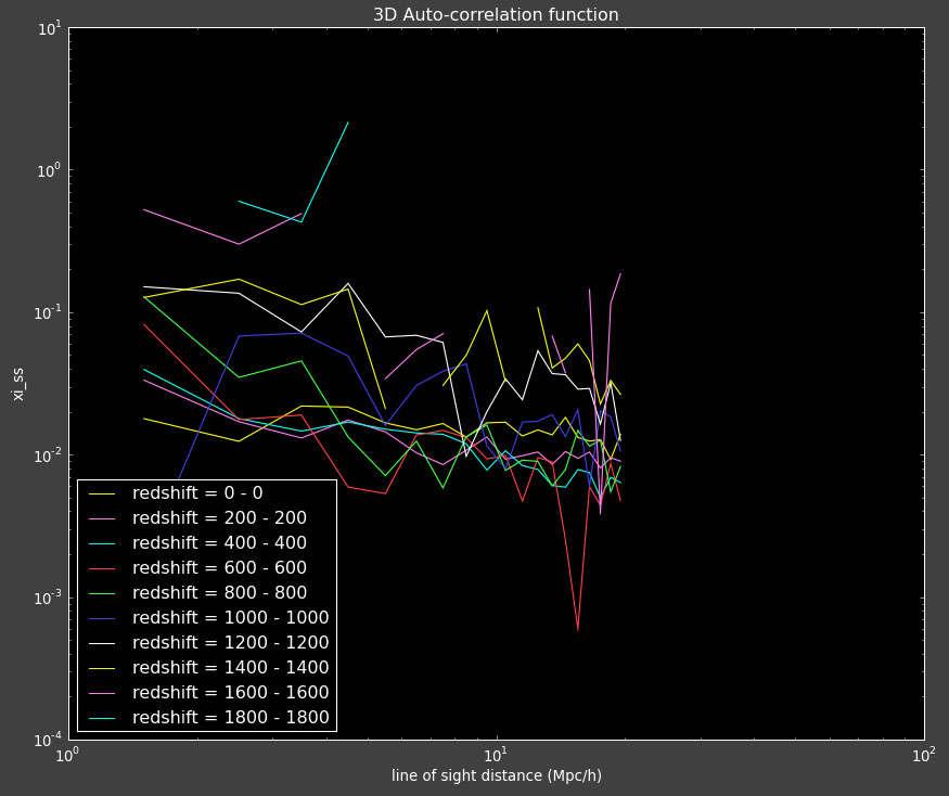
I'm running the reconstruction on the data. I'm doing in the working directory: .../pythonJess/run2010329_1319. I am running this with 12 redshift bins and 250k photometric and spectroscopic objects.

I did a little bit of thinking about the number of grids for the correlation function. There is the strange balance that you want the number of grids to be less than the number of particles, otherwise you might as well just correlate all possible pairs. You also want the spacing to be much bigger than the max correlation length, otherwise even by going out one grid length, you will unnecessarily correlate too many objects. I feel like this is a computer science problem, and perhaps Adam Pauls or Erin Sheldon would know the answer?

I played with this a bit (tried upping the grid points to 1000, and this took forever to run). For the 2D correlation function, I am correlating out to a distance of 0.34 (with a box size of 1). Maybe I don't need to correlate out to such a big angle? We could probably have as few as 10 grid points in each dimension if we are going out to this large of an angle. For the 3D correlation function, I am correlating out to a distance of 20 Mpc/h (with a box size of 2400 Mpc/h) so we need at least ~120 grid points in each dimension.

For the 3D correlation function, some of the larger redshift bins have very few objects in them, and if we have ~100³ or 10⁶ grid points then we are wasting time griding if we have less than 10³ points in each set.

Here are the results from the reconstruction I ran yesterday. It looks like I don't have enough points because the correlation functions are very noisy.

The reconstructions don't look good and are highly variable:

I'm running on a bigger data set now.

Plots for Joe (and Brandon)

Aside - A couple weeks ago Brandon Basso complained that my buzzing wasn't frequent enough. He requested more plots and perhaps an update on Adam's research. Well ask and you shall receive! Brandon this plot-heavy post is dedicated to you.

I am trying to understand why we seem to be missing objects around u-g = 0.8. Joe suggested I make the color plots in different redshift bins. So here we go. Warning, there are a lot of plots.

First, let me show you a temperature plots of the different luminosity functions. Below are color-color diagrams where the color of the points changes as a function of redshift in the following way:

dark red = 1.0 < z < 1.2
red = 1.2 < z < 1.4
orange red = 1.4 < z < 1.6
orange = 1.6 < z < 1.8
gold = 1.8 < z < 2.0
lawn green = 2.0 < z < 2.2
lime green =2.2 < z < 2.4
dark green = 2.4 < z < 2.6
teal = 2.6 < z < 2.8
dodger blue = 2.8 < z < 3.0
royal blue = 3.0 < z < 3.2
blue = 3.2 < z < 3.4
navy= 3.4 < z < 3.6
dark slate blue = 3.6 < z < 3.8
dark orchid = 3.8 < z < 4.0

As a reminder here are the luminosity functions I am using:

The above plot shows several luminosity functions.

Green is Richards 06, cyan is Jiang, purple is Jiang Combined (what we used in previous QSO Catalog, white is a Richard/Jiang average (suggested by Myers).

Here are the color-color redshift temperature plots for the QSO Catalogs generated by the above luminosity functions (click plots on below to make larger):

Also I have made color-color plots binned by redshift separately. I've done them for all of the luminosity functions, but they all look pretty much the same, so I'll just post them here for the Richards function (green luminosity function above), the redshift range is in the main title of the plots:

Here are some histograms of various quantities for the different luminosity functions the color scheme is same as above, Green is Richards 06, cyan is Jiang, purple is Jiang Combined (what we used in previous QSO Catalog, white is a Richard/Jiang average:

redshift

Color-band psffluxes


Color-band magnitudes

Color-color plot u-g/g-r

Hopefully that is enough plots for Joe to see what is going on with these QSO catalogs and Brandon to be satisfied.

Oh and here is an update on Adam's research (check out his shirt).

Parallelization

Adam rocks. He helped me figure out a way to parallelize the calculations of my correlation functions to that they all happen at once. Hopefully this will speed up my code by a factor of 10-20. Here is how it works:

A while ago I posted about how to use qsub to run scripts. I've now change my python code to call qsub within the program which calculates the correlation functions.

I have the following script:

runcrossCorr.script

~~~~~~~~~~~~~~

#PBS -l nodes=1

#PBS -N JessCC$job

#PBS -j oe

#PBS -m ea

#PBS -M jakirkpatrick@lbl.gov

#PBS -o qsub.out

cd /home/jessica/repository/ccpzcalib/Jessica/pythonJess

echo "$corr2dfile $argumentfile > $outfile"

$corr2dfile $argumentfile > $outfile

~~~~~~~~~~~~~~

this script is called using the following command:

qsub -v job=0, corr2dfile=./2dcorrFinal, argumentfile=./run2010129_237/wpsInputs0, outfile=./run2010129_237/wps0.dat runcrossCorr.script

where -v basically sets up environment variables for the qsub command so that within the script (in this example)

$job is replaced with 0

$corr2dfile is replaced with ./2dcorrFinal

$argumentfile is replaced with /run2010129_237/wpsInputs0

$outfile is replaced with ./run2010129_237/wps0.dat runcrossCorr.script

Many of these qsub commands can be run in python and they all are sent to the queue and run in parallel on different cluster computers.

I've done this so that python automatically changes the argumentfile and outfile and runs all the correlation functions at once.

These correspond to updated versions of my python functions runcrossCorr and runautoCorr in the correlationData library.

Look at all my jobs running (type qstat into terminal)!

And it even emails me when it's done!

So, now all I do is make a python script that runs all the code and set it going in the background:

python 100128run.py 100128.out 2> 100128.err &

I'm running with 1,000,000 points and finer redshift binning. Hopefully this will work even better!

SVM Results

I've been playing with using a support vector machine (SVM) for quasar target selection. Adam suggested this because it seem that the likelihood method was very similar to this already solved computer science problem. He helped me get SVM-light working using R.

The way this method works is that you input variable information for a set of training objects that represent what you are looking for (in this case quasars) and what you are not looking for (everything else).

I trained on the u-g-r-i-z fluxes (the same fluxes used to in the likelihood method) from the qso template and everything else (from now on referred to as everything) template objects. I tell SVM which are quasars and which are everything. It takes a long time to train the SVM, so I've been taking subsets of the quasar/everything catalogs to make the system faster (the likelihood uses ~1,000,000 objects).

I then take the human-confirmed truth table objects and run them through the SVM to classify as quasar or not. Below are the results:

Using 30,000 training qsos and 30,000 training stars
#quasars targeted
[1] 700
#not quasars not targeted
[1] 466
#quasars not targeted
[1] 255
#not quasars targeted
[1] 926
>
#Accuracy of targeting (qsos targeted / total targeted)
[1] 0.4305043

~~~

Using 100,000 training qsos and 100,000 training stars
#quasars targeted
[1] 709
#not quasars not targeted
[1] 480
#quasars not targeted
[1] 246
#not quasars targeted
[1] 912
>
#Accuracy of targeting (qsos targeted / total targeted)
[1] 0.4373843

~~~

Compared with the likelihood method:
#quasars targeted
[1] 793
#not quasars not targeted
[1] 908
#quasars not targeted
[1] 162
#not quasars targeted
[1] 484
>
#Accuracy of targeting (qsos targeted / total targeted)
[1] 0.620987

I can try adding in more information like the errors, or the likelihood values as additional vectors in this analysis, but it doesn't seem like it is working as well as the likelihood or that adding more objects improves accuracy very much (using ~3 times as many objects only increased the accuracy by >1%). I could run on larger training sets and see if this makes a difference too.

Big Box Results

Below are the resulting 3D correlation function from the run on the big box (described in previous blog post)

3D Correlation Functions on large mock data box

The first thing I notice is that they don't match as well as the functions matched on the smaller box. Following up on my concern from yesterday about the distribution of the random declinations:

The red line is the mock data and the blue line is the random data.

As you can see I am not properly simulating the declination randoms. Adam and I actually got in an argument/discussion about this on Tuesday. He was concerned that randomly populating in a ra, dec, redshift mask and then converting to x, y, z, was not the same as randomly populating in x, y, z but constraining the points to be within the mask. The above plot seems to point to this being true. My question is if this is also true with the Sloan data, or is the above an artifact of the fact that this mock data is actually in x, y, z coordinates, and I am applying a conversion/cut to try to simulate what is happening with the data. But with the Sloan data the true coordinate system is ra/dec/redshift, and so I would expect the point to be evenly distributed in that coordinate system, and slightly warped in x, y, z... but maybe this example shows I am wrong about this. Next step is to make these plots for Sloan data.

More worrying histograms:

Rage!

The reconstruction doesn't work.

I am so frustrated! I don't know what I am doing wrong. It doesn't match at all. I am having one of those moments where I feel like nothing I do ever works and I am a complete failure as a grad student. I mean, I'm in my 5th year of my PhD and don't have a single paper published, nor a working project. Everything that I am doing that does work is someone else's code (i.e. Alexia or David) and therefore has nothing to do with my talent or skills. Rage Rage Rage!

Here is a histogram of the "redshifts" (converted to units of comoving line-of-sight distance (Gpc/h) away from the observer) of the photometric data set (based on the Sloan photo-z's):

This is what the reconstruction should look like. However, when I do the reconstruction I get the following:

(The green is the reconstruction)

This actually paints a better picture than I actually have because

1) The normalization doesn't work and so I am tuning the normalization to match the answer (can't do this when I don't know the answer).

2) This is with really course binning. If I use finer binning (which is what we would ideally want to do), I get worse results:

What is up with the reconstruction going to zero (~1, 1.6, 1.9 Gpc/h)? I am so confused about that. Something that Adam and I discussed last night was that we would hope that this method would work at least as well as simply taking a histogram of the redshifts of the spectroscopic data set. In this case the spectroscopic data is actually from the same data as the photometric set, so the redshift distributions of the two sets are almost identical:

The fact that the reconstruction is significantly worse than this is really disheartening. I give up for today. I'm going to work on likelihood stuff in rebellion! (and post a sad facebook status message so people feel sorry for me and make me feel better)

Running Scripts

In science it seems that we are supposed to somehow organically learn how to use linux computers. I don't know how people do this. I feel like I know only 15 commands because I use them everyday. Everything else I need to do on linux I either have to ask others to help me, or I look it up when I need it and then promptly forget. All books on the subject seem to give me more information than I need. Is there a 'Practical Linux for Dummies' book?

However, one of the MANY benefits of dating a computer scientist (for those who haven't tried it, I highly recommend it) is that Adam knows how to do almost anything I would want to do on a computer. I've lost track of how many times he has helped me.

Latest example of this is running a script remotely the need to stay logged into the computer. I know this is a basic task, but every time I've tried to get someone to show me how to do it, I've never gotten a clear-cut answer.

So this is how I did it (I am writing it here so that I when I promptly forget how to do this, it will be easy to remind myself):

1) At the top of your python code put the following line (after the import statements):
if __name__ == '__main__':
For more info.

2) Indent the rest of your code (as python requires you to do for all functions)

3) Make sure your code doesn't plotting in it.

4) Save your code as a python script (i.e. code2run.py)

5) In a terminal window type the following:

> python code2run.py code2run.out 2> code2run.err &

6) Check that your code is running by typing the command: top

7) Now you can close your terminal window and come back to check on the run later by typing "top" again.

8) Any outputs to the terminal will go to the file code2run.out, and error messages will go to code2run.err

It would be nice if I could include in this script something where it would email me or send me some sort of message once the run is complete. Anyone know how to do this?

A Light Idea

I have been talking to Adam Pauls about this likelihood method for selecting quasars for BOSS in SDSS-III. He has suggested looking into this application: SVM-Light. SVM is a support vector machine. It is basically a well-establish classification system for multivariate systems. The interesting thing about this program is that I can not only use it to optimize the likelihood algorithm, but I can put in the results of other classification algorithms (we are also using neural net and KDE methods) and use those as additional "variables" in my system. I could also use additional information like sky position or photometric redshift to add weights to different objects. Adam is showing me how to use this, and I am hoping it will be useful for optimizing the selection codes.