Figuring out Mask Problems

I re-made the random catalogs without removing the duplicates. David thought that perhaps this was causing problems with the randoms not matching the catalogs or the correlation functions not working properly.

Below are a bunch of histograms of the distribution of the data (white) and randoms (green) for the two methods I have tried for making randoms, mine and Shirley's. You'll notice that the spectroscopic randoms mismatch the spectroscopic data much more than the photometric data/randoms (for both methods). This makes me perhaps think there is a problem with the mask I am using for the spectroscopic set. Martin White made this mask for me.. I've ask for a meeting with David this afternoon to look at this in more detail.

My randoms

Shirley's Randoms

I've tried zooming in on regions in the data where the mismatch is greatest. For instance ( dec > 40, 110 < ra < 130). I've posted these on the blog too.

It does look like there are regions where there are data and not randoms, which would suggest a problem with the mask. (Note that the regular spacing of the randoms is because this is how Shirley generates randoms, by putting an object in the center of the grid). I plotted these because it is easier to see with the regular spacing that regions have been missed. For instance at ra ~129.4, dec ~ 49.4, There are several data points (red), but but randoms (blue). You can click on the below pictures to make them bigger.

Making Randoms within Mask

I spent the weekend trying to make random catalogs inside the masks. They are taking forever to run, so I probably need to optimize better. I didn't spend too much time doing this before because I figured we would only need to make the random catalogs once and then we could just use them over and over again.

However, I've been running the code to generate them for > 13 hours and they still haven't finished, so there is a problem somewhere. The issue is that the mask represents a small region of the sky, but I am generating random objects over the whole sky, so 99.99% of the objects are rejected and thus the code is very inefficient.

Update: I found a bug in this code while trying to optimize explains why it was taking so long to run. Here is some testing about how it scales with number of randoms generated:

photo randoms:
500 randoms
Mon Dec 13 22:28:44 2010
Mon Dec 13 22:29:13 2010
29 seconds

5000 randoms
Mon Dec 13 22:34:00 2010
Mon Dec 13 22:31:02 2010
~3 minutes

50,000 randoms
Mon Dec 13 22:36:04 2010
Mon Dec 13 23:02:00 2010
~28 minutes

spectro randoms:
500 randoms
Mon Dec 13 22:32:10 2010
Mon Dec 13 22:31:45 2010
25 seconds

5000 randoms
Mon Dec 13 22:37:06 2010
Mon Dec 13 22:34:38 2010
~2.5 minutes

50,000 randoms
Mon Dec 13 22:38:51 2010
Mon Dec 13 23:01:42 2010
~23 minutes

The way the code works in it's current (inefficient) form:

For Spectroscopic Data:
1) Read in the two masks.
2) Create random ra and dec that are 5X as big as the spectro data set
3) Assign a redshift from the redshifts of the spectro data set (to keep same redshift distribution)
4) See if ra/dec is in the both masks
5) If it is in both masks, look at the weight in the BOSS mask. Assign a random weight to the object (between 0 and 1), if it is less than or equal to the weight of the BOSS mask then it is "observed", if it is greater than the BOSS weight it "isn't observed"
6) Repeat above until you reached the right number of randoms

For Photometric Data:
1) Read in the two masks.
2) Create random ra and dec that are 5X as big as the photo data set
3) See if ra/dec is in the both masks
4) Repeat above until you reached the right number of randoms

We don't need to assign a redshift to the photo data or "observe or not observe" because the photometric data doesn't have weights.

The code is here:

../pcode/photorandoms.pro
../pcode/spectrorandoms.pro

The code to run this as a qsub is here:
../pcode/makeRphoto.script
../pcode/makeRspec.script

You run it with the following code:
qsub makeR[photo,spec].script

The randoms have the same distribution as the data, shown in the following histograms, white is the data, red is the randoms:



Sweet!

No Overlap Data

I realized that I need to make sure that the photometric and spectroscopic data doesn't overlap. I've written code to do this here:

../pcode/removeDataOverlap.pro
../pcode/getSpectroPhotoData.pro

And the overlapping data is here:
/home/jessica/boss/spectroRaDecZMaskedNoOverLap.dat
/home/jessica/boss/photoRaDecZMaskedNoOverLap.dat

This is what we should use for the reconstruction.

Using the Whole Footprint with Masks

For the past few days I've been working on using masks to run correlation functions on the whole BOSS footprint. It's required learning how to use polygon masks and also to create randoms in these masks. Here is the code/testing:

To mask BOSS data (spectroscopic set)

;Read in BOSS data
bossgalaxies = '/home/jessica/boss/spAll-v5_4_14.fits'
spall = mrdfits(bossgalaxies, 1)

;Trim BOSS data to be a galaxy (remove QSOs, starts, etc)
isgal = where(spall.specprimary EQ 1 $
AND (spall.boss_target1 AND 2L^0+2L^1+2L^2+2L^3+2L^7) NE 0 $
AND strmatch(spall.class,'GALAXY*') $
AND spall.zwarning EQ 0)

;Select galaxies
galaxies = spall[isgal]
ra = galaxies.ra
dec = galaxies.dec
z = galaxies.z

;Select objects in the masks
weights = maskdataboth(ra,dec,z)

; Readout ra, dec, redshift of spectroscopic objects inside mask
thisfile = '/home/jessica/boss/spectroRaDecZMasked.dat'
writecol,thisfile,ra,dec,z

The code for maskdataboth is here:
/home/jessica/repository/ccpzcalib/Jessica/pythonJess/maskdataboth.pro

'maskdataboth' filters the data through both the BOSS mask and Shirley's mask to make sure the data sets are in the same ra/dec footprint.


To Mask Shirley's Data (photometric set)

;Read in Shirley's Photometric Data
file1 = "/home/shirleyho/research/SDSS_PK/powerspec_dir/DATA/ra_dec_z_run_rerun_camcol.z_gt_0.01"
readcol, file1, pra, pdec, pz, RUN, rerun, camcol, x, x, x, x, x, x, x, x, format='(F,F,F,D,D,D,D,D,F,F,F,F,F,F)'

;Select objects in the masks
pweights = maskdataboth(pra,pdec,pz)

; Readout ra, dec, redshift of spectroscopic objects inside mask
thisfile = '/home/jessica/boss/photoRaDecZMasked.dat'
writecol,thisfile,pra,pdec,pz

Here are plots of the data sets to show that they do indeed fall in the same region of the sky:




Both these data sets are saved in the following directory: /home/jessica/boss/
The code to run this is here: ../logs/101210log.pro

BOSS Galaxies

Spent today getting the BOSS Galaxies in the correct form to use as my spectroscopic data set. Here's what I did:

1) Downloaded latest spAll file from here to ~/boss/:
:/clusterfs/riemann/

raid006/bosswork/groups/boss/spectro/redux/spAll-v5_4_14.fits

2) In IDL, trim the data to be galaxies in stripe 82:
bossgalaxies = '/home/jessica/boss/spAll-v5_4_14.fits'
spall = mrdfits(bossgalaxies, 1)

stripe82gal = where(((spall.ra LE 60.0) OR (spall.ra GE 300.)) $
and ((spall.dec GE -1.25) and (spall.dec LE 1.25)) $
AND spall.specprimary EQ 1 $
AND (spall.boss_target1 AND 2L^0+2L^1+2L^2+2L^3+2L^7) NE 0 $
AND strmatch(spall.class,'GALAXY*') $
AND spall.zwarning EQ 0

3) Write these galaxies out to a col delimited file that python can read:
thisfile = '/home/jessica/boss/BOSSstripe82RaDec.dat'
writecol, thisfile, spall[stripe82gal].ra, spall[stripe82gal].dec, spall[stripe82gal].z

4) Do the same to Shirley Ho's photometric LRG file:
shirleydata = "/home/shirleyho/research/SDSS_PK/powerspec_dir/DATA/ra_dec_z_run_rerun_camcol.z_gt_0.01"
readcol, shirleydata, RA, DEC, z, RUN, rerun, camcol, x, x, x, x, x, x, x, x, format='(F,F,F,D,D,D,D,D,F,F,F,F,F,F)'
datasize = n_elements(ra)

;Data just within stripe 82
stripe82all = where(((ra LE 60.0) OR (ra GT 305.)) $
and ((dec GE -1.25) and (dec LE 1.25)))

; Readout ra, dec, redshift of stripe 82 Shirly objects
thisfile = '/home/jessica/boss/ShirlyDataRaDec.dat'
writecol, thisfile, ra[stripe82all], dec[stripe82all], z[stripe82all]

If I want to use the whole BOSS Galaxy footprint I have a mask here from Martin White:
/home/jessica/boss/bossX.002.ply

You can read this file like so:

infile = "./bossX.002.ply"
read_mangle_polygons, infile, polygons, id

There are more functions in idlutils in playing with the mask.

Now I am trying to do the reconstruction on these two data sets. Using BOSS as the spectroscopic set and Shirley's LRG galaxies as the spectroscopic galaxies.

Here are some plots of the two sets of data:

The log file to make these data files and plots is here:
../logs/101207log.pro
../logs/101207log.py

Data Run

I'm running the reconstruction on the data. I'm doing in the working directory: .../pythonJess/run2010329_1319. I am running this with 12 redshift bins and 250k photometric and spectroscopic objects.

I did a little bit of thinking about the number of grids for the correlation function. There is the strange balance that you want the number of grids to be less than the number of particles, otherwise you might as well just correlate all possible pairs. You also want the spacing to be much bigger than the max correlation length, otherwise even by going out one grid length, you will unnecessarily correlate too many objects. I feel like this is a computer science problem, and perhaps Adam Pauls or Erin Sheldon would know the answer?

I played with this a bit (tried upping the grid points to 1000, and this took forever to run). For the 2D correlation function, I am correlating out to a distance of 0.34 (with a box size of 1). Maybe I don't need to correlate out to such a big angle? We could probably have as few as 10 grid points in each dimension if we are going out to this large of an angle. For the 3D correlation function, I am correlating out to a distance of 20 Mpc/h (with a box size of 2400 Mpc/h) so we need at least ~120 grid points in each dimension.

For the 3D correlation function, some of the larger redshift bins have very few objects in them, and if we have ~100³ or 10⁶ grid points then we are wasting time griding if we have less than 10³ points in each set.

Here are the results from the reconstruction I ran yesterday. It looks like I don't have enough points because the correlation functions are very noisy.

The reconstructions don't look good and are highly variable:

I'm running on a bigger data set now.

Back on Track

I fixed the angular correlation function using the method outlined in my last post. I did a run again on the mock data using photometric and spectroscopic sets with 200,000 objects. The correlation functions look much better now (and the code runs much faster too!):

2D and 3D correlation functions

The 2D are actual angular separations (different from what Alexia was doing which was collapsing the third dimension onto a projection plane). This is super exciting because the noise has gone down a lot compared to what I was getting before. Hopefully this will mean a better reconstruction.

The distribution functions I applied to the two data sets are below:

The cyan line is a histogram of the number photometric objects as a function of comoving distance away from the observer. The magenta line is the imposed photometric distribution function (what we are trying to reconstruct). The green line is a histogram of the number of spectroscopic objects as a function of comoving distance away from the observer. Note that it is different than the photometric distribution.

And here is the reconstruction:

The magenta is the imposed distribution function (same as the previous plot) and the red is the reconstructed distribution. They look pretty much the same. Awesome.

1M Reconstruction

I ran a big reconstruction on the CAS data using 1,000,000 objects, and 20 redshift bins. The correlation functions at the lower redshifts (less than 720 Mpc/h) have much less noise:


But the correlation functions at larger redshifts look pretty noisy:

Perhaps I should bin so that I have a constant number of objects per bin instead of by equal redshift bins.

When I do the reconstruction, I get puzzling results:

The reconstruction seems to think there are a large number of points at redshift > 1.0 which aren't there. This could be due to low statistics at these redshifts and so the reconstruction just isn't working properly. The number of spectroscopic objects per bin is as follows:

0-120 Mpc/h: 14597 galaxies in spectroscopic dataset
120-240 Mpc/h: 45954 galaxies in spectroscopic dataset
240-360 Mpc/h: 55489 galaxies in spectroscopic dataset
360-480 Mpc/h: 59451 galaxies in spectroscopic dataset
480-600 Mpc/h: 64381 galaxies in spectroscopic dataset
600-720 Mpc/h: 56290 galaxies in spectroscopic dataset
720-840 Mpc/h: 55916 galaxies in spectroscopic dataset
840-960 Mpc/h: 49536 galaxies in spectroscopic dataset
960-1080 Mpc/h: 29109 galaxies in spectroscopic dataset
1080-1200 Mpc/h: 20852 galaxies in spectroscopic dataset
1200-1320 Mpc/h: 16729 galaxies in spectroscopic dataset
1320-1440 Mpc/h: 13715 galaxies in spectroscopic dataset
1440-1560 Mpc/h: 8969 galaxies in spectroscopic dataset
1560-1680 Mpc/h: 5094 galaxies in spectroscopic dataset
1680-1800 Mpc/h: 2374 galaxies in spectroscopic dataset
1800-1920 Mpc/h: 890 galaxies in spectroscopic dataset
1920-2040 Mpc/h: 381 galaxies in spectroscopic dataset
2040-2160 Mpc/h: 169 galaxies in spectroscopic dataset
2160-2280 Mpc/h: 85 galaxies in spectroscopic dataset
2280-2400 Mpc/h: 16 galaxies in spectroscopic dataset

It looks like I shouldn't use bins greater than ~1Mpc/h for the reconstruction because we have so few galaxies out there. If I try doing the reconstruction only using bins up to 1080 Mpc/h this is that I get:

There seems to be a problem at the earlier redshifts, perhaps due to low statistics in the first redshift bin? But the reconstruction looks sort of good.

I'm need to see what Alexia thinks about this "forcing to zero" issue at the edges. I also want to try this with the LRG catalog. I'm going to set a run going where I bin such that there are constant numbers of galaxies per bin, not constant redshifts. Alexia, let's chat tomorrow early?

Housekeeping

I've restructured the way the code is run to that I can do multiple runs at once and to hopefully make it easier to re-produce runs and look at older runs quickly. Below is how it works.

Whenever I do a new run, the first thing that python does is create a new 'working directory' of the following format:

runYYYYMD_HM

where
YYYY is the year (2010)
M is the month (2)
D is the day (1)
H is the hour (1337)
so in this example the directory would be called: run201021_1337

This in done in python by the following code:

now = dt.datetime.now()
year = now.year
month = now.month
day = now.day
hour = now.hour
minute = now.minute
workingDir = "run%d%d%d_%d%d"%(year,month,day,hour,minute)
command = "mkdir "+ workingDir
os.system(command)

Within this directory all the photometric and spectroscopic data files are placed for each of the redshift bins. These files are in the format:

photo2D.dat - ra and dec of all photometric data
spec2D_#.dat - ra and dec of the spectroscopic data in the # redshift bin
spec3D_#.dat - x, y, z of the spectroscopic data in the # redshift bin
photoCD.dat - the comoving distance of the photometric data (from photo-zs)

I then compute the 2D cross correlation functions between the photo2D.dat and spec2D_#.dat files and these are saved in the wps#.dat files. The input arguments for these correlation functions are in the files wpsInputs#.

I then compute the 3D auto correlation functions on the spec3D_#.dat files and these are saved in the xiss#.dat files. The input arguments for these correlation functions are in the files xiInputs#.

Because the correlation functions in each redshift bin are submitted as qsub jobs, they take a while to run... so at this point you need to wait for all those jobs to finish. The jobs are named as follows:

2D Cross Correlation: JessWps#workingDir
3D Auto Correlation: JessXiss#workingDir

where # is the redshift bin and workingDir is the name of the working directory.

I can monitor the qsub jobs by typing in 'qstat' to see what is running. Once all the jobs for my working directory are completed then I do the following:

load in the constants from the run file (I put this in the working directory) and it is named YYMMDD_#run.py

where YY is the year (10)
MM is the month (02)
and DD is the day (01)
# is the run number (if I've done multiple runs on this day)

I set the variable workingDir to the working directory.

I load in the photometric comoving distances (which are saved in a file called photoCD.dat):

photoCD = readPhotoCDfile(photoCDfile)

I create the wps and xi matrixes (which are used in the reconstruction) and save them as files:

wpsMat.dat and xiMat.dat respectively.

Then I can do the reconstruction of the redshift distribution and compare it to the photoCD.

Correlation Correlation

Here are the angular cross correlation between the photometric data set and the binned spectroscopic data sets (12 -- one for each bin):

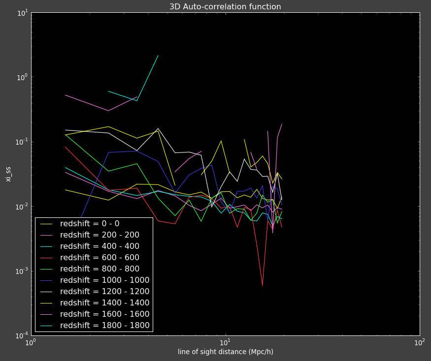
I also calculate the 3D auto-correlation function of spectroscopic data with itself (12 -- one for each bin):

The 3D correlation functions don't look very good to me. I would expect them to have a similar shape to the 2D correlation function, but I actually had to plot these on a normal plot (not log-log) because they were going negative. Alexia -- what do these look like for you on the mock data? I guess I should calculate them on the mock data myself.

Next step, reconstruction...

Talking with Weinberg

I ran into David Weinberg at tea at the IAS today. We started talking about the Newman Project.
He suggested that after we get the method working on Stripe 82 using the LRGs as our "spectroscopic sample" and the rest of the galaxies as our "photometric sample" we could compare the reconstructed distribution with spectroscopic "follow-up" surveys such as COSMOS, Vimas?, and DEEP.

Then it would be interesting to break down the main sample (i.e. the rest of the galaxies) by colors and do redshift distribution reconstruction on each type of galaxy. We could also break these into photometric redshift slices and then look at the reconstruction in each slice and break those down by colors, to see if perhaps there is a different spread in the colors.

I thought these were really good ideas and ones that I haven't though of before. Need to talk to Schlegel/Nikhil and see what they think. Oh exciting!