Changing QSO Catalog Inputs

I'm trying to figure out how to modify the inputs (currently SDSS DR5 quasars with good photometry) into Joe's Monte Carlo. Here is what I have figured out so far (all the below files are on riemann):

hiz_kde_numerator.pro ;main program to generate the QSO Catalog
(calls) →
qso_fakephoto.pro ;generates simulated redshift and i-magnitude based on luminosity function and DR5 inputs
(calls) →
qso_photosamp.pro ;This generates the training set photometry
(calls) →
sdss_read_data.pro ;This reads in SDSS data it currently has the following 'DR5' call
qsos = sdss_read_data('DR5', Z_MIN = Z_MIN, Z_MAX = Z_MAX)

Here is a color-color redshift temperature plot of these DR5 QSOs:


I'm going to try to add in the BOSS QSOs with co-added photometry, especially in the redshift range z > 2.0 where we seem to be missing QSOs:


I found that there are 1,973 BOSS quasars that have a redshift above 2.0 for which we also have coadded photometry. Here they are plotted:


While it is a little more filled in in the u-g = 0.8 space, comparing it to all the BOSS quasars (regardless of how good their photometry is) below:

Comparing Quasars

Here are the color-color diagrams with redshift temperature plots for the current QSO Catalog (in the BOSS redshift range) and the BOSS 3PC Quasars (same temperature-z map as before). I think this shows pretty well that something is wrong with the QSO Catalog's color distribution. These both have the same number of quasars, in the same redshift range:

Their redshift distributions are not that different so this is really a matter of the input QSOs not properly representing the spread of the possible colors, I believe:

White is BOSS QSOs, Green is the QSO Catalog.
The histograms are scaled as a percentage in each bin.

I want to add in BOSS QSOs to Joe's Monte Carlo. We can do this by just adding in the "chunk 1" objects where we have co-added photometry from Stripe-82, or we can apply the same cuts in terms of brightness as we did to the DR5 catalog.

Plots for Joe (and Brandon)

Aside - A couple weeks ago Brandon Basso complained that my buzzing wasn't frequent enough. He requested more plots and perhaps an update on Adam's research. Well ask and you shall receive! Brandon this plot-heavy post is dedicated to you.

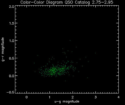
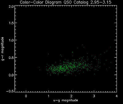
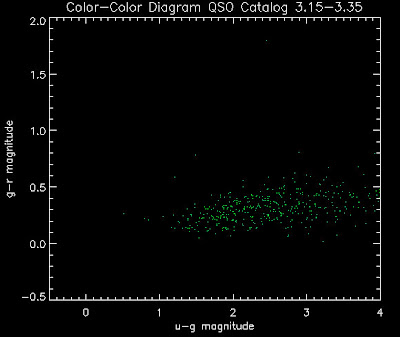
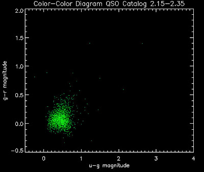
I am trying to understand why we seem to be missing objects around u-g = 0.8. Joe suggested I make the color plots in different redshift bins. So here we go. Warning, there are a lot of plots.

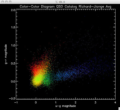
First, let me show you a temperature plots of the different luminosity functions. Below are color-color diagrams where the color of the points changes as a function of redshift in the following way:

dark red = 1.0 < z < 1.2
red = 1.2 < z < 1.4
orange red = 1.4 < z < 1.6
orange = 1.6 < z < 1.8
gold = 1.8 < z < 2.0
lawn green = 2.0 < z < 2.2
lime green =2.2 < z < 2.4
dark green = 2.4 < z < 2.6
teal = 2.6 < z < 2.8
dodger blue = 2.8 < z < 3.0
royal blue = 3.0 < z < 3.2
blue = 3.2 < z < 3.4
navy= 3.4 < z < 3.6
dark slate blue = 3.6 < z < 3.8
dark orchid = 3.8 < z < 4.0

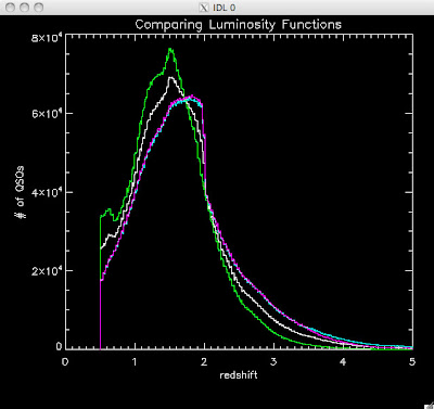
As a reminder here are the luminosity functions I am using:

The above plot shows several luminosity functions.

Green is Richards 06, cyan is Jiang, purple is Jiang Combined (what we used in previous QSO Catalog, white is a Richard/Jiang average (suggested by Myers).

Here are the color-color redshift temperature plots for the QSO Catalogs generated by the above luminosity functions (click plots on below to make larger):

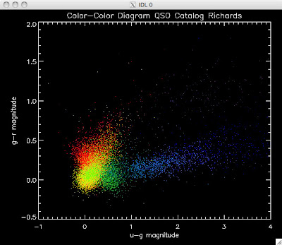
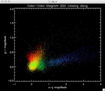
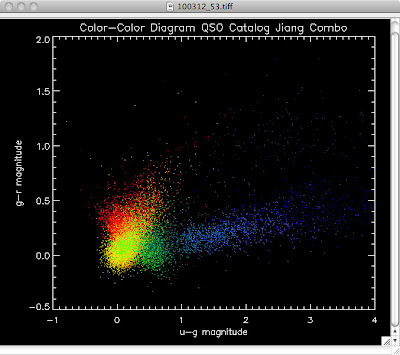
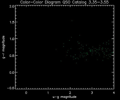
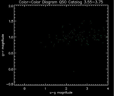
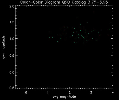
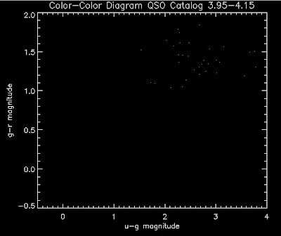
Also I have made color-color plots binned by redshift separately. I've done them for all of the luminosity functions, but they all look pretty much the same, so I'll just post them here for the Richards function (green luminosity function above), the redshift range is in the main title of the plots:

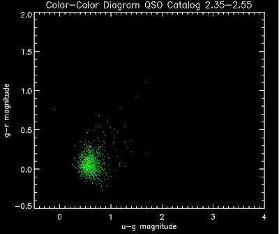
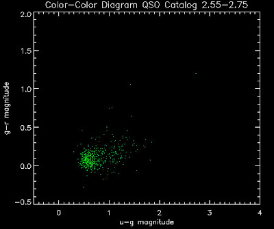
Here are some histograms of various quantities for the different luminosity functions the color scheme is same as above, Green is Richards 06, cyan is Jiang, purple is Jiang Combined (what we used in previous QSO Catalog, white is a Richard/Jiang average:

redshift

Color-band psffluxes


Color-band magnitudes

Color-color plot u-g/g-r

Hopefully that is enough plots for Joe to see what is going on with these QSO catalogs and Brandon to be satisfied.

Oh and here is an update on Adam's research (check out his shirt).

Likely Testing

I'm trying to track down why the likelihood method is missing quasars that other targeting methods are finding.

The plot of human-confirmed QSOs that were in the target list for the likelihood method. The magenta are targeted by likelihood, the cyan are missed by likelihood, the white are targeted only by likelihood (click on image to enlarge):

Color-Color (u-g vs g-r)
of likelihood selected objects (magenta),
likelihood missed objects (cyan),
likelihood only objects (white)

The reason this plot looks different than yesterdays is because I was accidentally plotting both QSOs and stars on the plot yesterday. The above human-confirmed QSOs.

Below is a log-log plot of the likelihood selection variables L_everything vs L_qso for the likelihood-selected QSOs (magenta), the likelihood-missed QSOs (cyan), the likelihood-selected stars (red), and the likelihood-missed stars (green) you can see the value of L_ratio we cut on is the slope of the dividing line between these populations (click on image to enlarge):

L_everything vs L_qso

I've looked at the individual fluxes of the likelihood selected/missed QSOs to see if there an obvious place in flux-color space where we can get more of the missing objects. They are all intermixed.

David Schlegel suggested increasing the 'added errors' in the likelihood calculation to see if this improves things. I am re-running the likelihoods on these ~1400 objects (above) with larger errors. The hope is that because we are have such a sparse sample of the QSOs, that by increasing the errors we'll allow for objects that are "farther away" in flux-space to be selected. The errors are currently on the order of ~1%. I am re-running with 10%, however David suggests that I do it with 5%, so I'll run with that too.

Back to the Likelihoods

It's been a while since I have worked on the likelihood QSO selection method. With the next deadline for target selection is coming up, it's time to go "Back to the Likelihoods." Note to self: It more time efficient to keep working on something continuously than to not work on it for weeks and then waste a day trying to remember what I was doing.

Where we left off...
Below is a color-color (ug - gr) plot of the final likelihood selection objects for the commissioning data.

The white data points are a random sampling of 20,000 possible objects to target. The red data points are objects who's likelihood ratio is greater than 0.1, where likelihood ratio is defined as:

where L_QSO and L_everything, as described in "A Likely Result" are defined as:

The green data points are objects are objects who's likelihood ratio is greater than 0.1 and L_everything is greater than 10^-6. This is eliminate classification of "fringe" objects that are not close to any objects (and therefore have a small everything likelihood.

The likelihood was then run on the co-added Stripe 82 data and all of the above green objects were submitted as targets for the commissioning data.

What we need to work out...

• Why are the likelihoods so small/large? The likelihoods should be a probability, but we have likelihood's spanning from 0-11.
  
• Why is our completeness and efficiency on the MMT data so poor?
• How does the likeliness compare to QSOs based on variability?
• How well does this method work on single epoch Stripe 82 data versus the co-added images?