SDSS-III Publication 33: A Simple Likelihood Estimator for Quasar Target Selection
Authors: Jessica A. Kirkpatrick (corresponding author)
David J. Schlegel, Nicholas P. Ross, Adam D. Myers, Joseph F. Hennawi
Abstract:
We present a new method for quasar target selection using a likelihood estimator. For our purposes we target quasars using Sloan Digital Sky Survey (SDSS) photometry to a magnitude limit of g=22. The efficiency and completeness of this technique is measured using Baryon Oscillation Spectroscopic Survey (BOSS) Commissioning Data, taken in late 2009. This technique was used as the CORE method for target selection for BOSS Year 1 spectroscopy to be realized in the 9th SDSS data release (DR9). When targeting at a density of 40 objects/deg2 we find the efficiency of this technique to be 41% and the completeness compared to all quasars identified in BOSS Commissioning Data to be 62%. This paper also describes possible extensions and improvements for this technique.
Comments:
SDSS-III participants have three weeks to send comments and to request changes. Participants comments should be sent to the Jessica Kirkpatrick.
The deadline to submit comments is Wednesday, April 6th 2011.
This is a BOSS science paper intended for submission to the Astrophysical Journal.
Downloads:
The most up to date .pdf of the paper can be found here:
likelihood paper (current) this version will be updated as I receive comments during the next three weeks.
The version of the paper submitted to the collaboration (3/16) is here:
likelihood collaboration submission
There is also a single column, double spaced version here (for easier editing):
likelihood paper one column
The .tex files and all associated figures, can be checked-out from the SVN at this location:
svn co svn+ssh://sdss3svn@sdss3.org/repo/boss/bosstarget/trunk/tex/likelihood/
Or downloaded here on the SDSS3 wiki.
Showing posts with label target selection. Show all posts
Showing posts with label target selection. Show all posts
Wednesday, March 16, 2011


Monday, March 15, 2010
Useful IDL Commands
I need to do some work for the likelihood project and thus code in IDL again. Because I am not working in IDL very frequently, I tend to forgot commands and syntax. I thought it would be useful to compile a list of commands here so that I don't have to keep looking these up again and again.
number of elements in an array:
print, N_ELEMENTS(array)
unix command in idl: dollar sign ($) before command
$pwd
$ls
list all variables currently being used:
help
doc_library, 'spherematch' -- man page for the function
which, 'spherematch' --- tells you where in the IDL path the function is.
when recompiling idlutils need to use evilmake
!pi is constant pi
plothist (makes histogram plot)
when looking at a structure you use the /str command:
help, mystructure, /str
reading a fits file using mrdfits:
filedata = mrdfits(file2read, 1)
Combine two structures of the same size:
struct3 =struct_combine(struct1,struct2)
Concatenate two structure of the same type:
struct3 = [struct1, struct2]
Plotting Histogram (from here):
total with higher precision: total(...., /double)
in for loops:
for j = 0L, rsize-1 do begin
the L makes j a long int.
;Show color table
colorName = PickColorName(startColorName)
; Make heat map (warning, not very sophisticated)
colorobject = qsotemplate1.z_sim
xobject = ugqcolor1
yobject = grqcolor1
colorbin = 0.3
colorstart = 1.0
colorstop = colorstart + colorbin
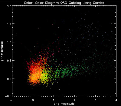
plot, xobject[0:1], yobject[0:1], ps=null, color=fsc_color('white'), xr=[-0.5,4],yr=[-0.5,2], XTITLE = 'u-g magnitude', YTITLE = 'g-r magnitude', TITLE = 'Color-Color Diagram QSO Catalog Jiang Combo', charsize = 1.5, charthick = 1
zrange = where(colorobject GE colorstart AND colorobject LT colorstop)
oplot, xobject[zrange], yobject[zrange], ps=3, color=FSC_COLOR('dark red') ;Fake QSOs
colorstart = colorstop
colorstop = colorstart + colorbin
zrange = where(colorobject GE colorstart AND colorobject LT colorstop)
oplot, xobject[zrange], yobject[zrange], ps=3, color=FSC_COLOR('red') ;Fake QSOs
colorstart = colorstop
colorstop = colorstart + colorbin
zrange = where(colorobject GE colorstart AND colorobject LT colorstop)
oplot, xobject[zrange], yobject[zrange], ps=3, color=FSC_COLOR('orange red') ;Fake QSOs
colorstart = colorstop
colorstop = colorstart + colorbin
zrange = where(colorobject GE colorstart AND colorobject LT colorstop)
oplot, xobject[zrange], yobject[zrange], ps=3, color=FSC_COLOR('orange') ;Fake QSO
colorstart = colorstop
colorstop = colorstart + colorbin
zrange = where(colorobject GE colorstart AND colorobject LT colorstop)
oplot, xobject[zrange], yobject[zrange], ps=3, color=FSC_COLOR('gold') ;Fake QSOs
colorstart = colorstop
colorstop = colorstart + colorbin
zrange = where(colorobject GE colorstart AND colorobject LT colorstop)
oplot, xobject[zrange], yobject[zrange], ps=3, color=FSC_COLOR('lawn green') ;Fake QSOs
colorstart = colorstop
colorstop = colorstart + colorbin
zrange = where(colorobject GE colorstart AND colorobject LT colorstop)
oplot, xobject[zrange], yobject[zrange], ps=3, color=FSC_COLOR('lime green') ;Fake QSOs
colorstart = colorstop
colorstop = colorstart + colorbin
zrange = where(colorobject GE colorstart AND colorobject LT colorstop)
oplot, xobject[zrange], yobject[zrange], ps=3, color=FSC_COLOR('dark green') ;Fake QSOs
colorstart = colorstop
colorstop = colorstart + colorbin
zrange = where(colorobject GE colorstart AND colorobject LT colorstop)
oplot, xobject[zrange], yobject[zrange], ps=3, color=FSC_COLOR('teal') ;Fake QSOs
colorstart = colorstop
colorstop = colorstart + colorbin
zrange = where(colorobject GE colorstart AND colorobject LT colorstop)
oplot, xobject[zrange], yobject[zrange], ps=3, color=FSC_COLOR('dodger blue') ;Fake QSOs
colorstart = colorstop
colorstop = colorstart + colorbin
zrange = where(colorobject GE colorstart AND colorobject LT colorstop)
oplot, xobject[zrange], yobject[zrange], ps=3, color=FSC_COLOR('royal blue') ;Fake QSOs
colorstart = colorstop
colorstop = colorstart + colorbin
zrange = where(colorobject GE colorstart AND colorobject LT colorstop)
oplot, xobject[zrange], yobject[zrange], ps=3, color=FSC_COLOR('blue') ;Fake QSOs
colorstart = colorstop
colorstop = colorstart + colorbin
zrange = where(colorobject GE colorstart AND colorobject LT colorstop)
oplot, xobject[zrange], yobject[zrange], ps=3, color=FSC_COLOR('navy') ;Fake QSOs
colorstart = colorstop
colorstop = colorstart + colorbin
zrange = where(colorobject GE colorstart AND colorobject LT colorstop)
oplot, xobject[zrange], yobject[zrange], ps=3, color=FSC_COLOR('dark slate blue') ;Fake QSOs
colorstart = colorstop
colorstop = colorstart + colorbin
zrange = where(colorobject GE colorstart AND colorobject LT colorstop)
oplot, xobject[zrange], yobject[zrange], ps=3, color=FSC_COLOR('dark orchid') ;Fake QSOs
number of elements in an array:
print, N_ELEMENTS(array)
unix command in idl: dollar sign ($) before command
$pwd
$ls
list all variables currently being used:
help
doc_library, 'spherematch' -- man page for the function
which, 'spherematch' --- tells you where in the IDL path the function is.
when recompiling idlutils need to use evilmake
!pi is constant pi
plothist (makes histogram plot)
when looking at a structure you use the /str command:
help, mystructure, /str
reading a fits file using mrdfits:
filedata = mrdfits(file2read, 1)
Combine two structures of the same size:
struct3 =struct_combine(struct1,struct2)
Concatenate two structure of the same type:
struct3 = [struct1, struct2]
Plotting Histogram (from here):
PRO t_histogramIf you add maxmatch=1 to your spherematch it will avoid duplicates (should default to this)
data = [[-5, 4, 2, -8, 1], $
[ 3, 0, 5, -5, 1], $
[ 6, -7, 4, -4, -8], $
[-1, -5, -14, 2, 1]]
hist = HISTOGRAM(data)
bins = FINDGEN(N_ELEMENTS(hist)) + MIN(data)
PRINT, MIN(hist)
PRINT, bins
SPLOT, bins, hist, YRANGE = [MIN(hist)-1, MAX(hist)+1], PSYM = 10, XTITLE = 'Bin Number', YTITLE = 'Density per Bin'
END
total with higher precision: total(...., /double)
in for loops:
for j = 0L, rsize-1 do begin
the L makes j a long int.
;Show color table
colorName = PickColorName(startColorName)

; Make heat map (warning, not very sophisticated)

colorobject = qsotemplate1.z_sim
xobject = ugqcolor1
yobject = grqcolor1
colorbin = 0.3
colorstart = 1.0
colorstop = colorstart + colorbin
plot, xobject[0:1], yobject[0:1], ps=null, color=fsc_color('white'), xr=[-0.5,4],yr=[-0.5,2], XTITLE = 'u-g magnitude', YTITLE = 'g-r magnitude', TITLE = 'Color-Color Diagram QSO Catalog Jiang Combo', charsize = 1.5, charthick = 1
zrange = where(colorobject GE colorstart AND colorobject LT colorstop)
oplot, xobject[zrange], yobject[zrange], ps=3, color=FSC_COLOR('dark red') ;Fake QSOs
colorstart = colorstop
colorstop = colorstart + colorbin
zrange = where(colorobject GE colorstart AND colorobject LT colorstop)
oplot, xobject[zrange], yobject[zrange], ps=3, color=FSC_COLOR('red') ;Fake QSOs
colorstart = colorstop
colorstop = colorstart + colorbin
zrange = where(colorobject GE colorstart AND colorobject LT colorstop)
oplot, xobject[zrange], yobject[zrange], ps=3, color=FSC_COLOR('orange red') ;Fake QSOs
colorstart = colorstop
colorstop = colorstart + colorbin
zrange = where(colorobject GE colorstart AND colorobject LT colorstop)
oplot, xobject[zrange], yobject[zrange], ps=3, color=FSC_COLOR('orange') ;Fake QSO
colorstart = colorstop
colorstop = colorstart + colorbin
zrange = where(colorobject GE colorstart AND colorobject LT colorstop)
oplot, xobject[zrange], yobject[zrange], ps=3, color=FSC_COLOR('gold') ;Fake QSOs
colorstart = colorstop
colorstop = colorstart + colorbin
zrange = where(colorobject GE colorstart AND colorobject LT colorstop)
oplot, xobject[zrange], yobject[zrange], ps=3, color=FSC_COLOR('lawn green') ;Fake QSOs
colorstart = colorstop
colorstop = colorstart + colorbin
zrange = where(colorobject GE colorstart AND colorobject LT colorstop)
oplot, xobject[zrange], yobject[zrange], ps=3, color=FSC_COLOR('lime green') ;Fake QSOs
colorstart = colorstop
colorstop = colorstart + colorbin
zrange = where(colorobject GE colorstart AND colorobject LT colorstop)
oplot, xobject[zrange], yobject[zrange], ps=3, color=FSC_COLOR('dark green') ;Fake QSOs
colorstart = colorstop
colorstop = colorstart + colorbin
zrange = where(colorobject GE colorstart AND colorobject LT colorstop)
oplot, xobject[zrange], yobject[zrange], ps=3, color=FSC_COLOR('teal') ;Fake QSOs
colorstart = colorstop
colorstop = colorstart + colorbin
zrange = where(colorobject GE colorstart AND colorobject LT colorstop)
oplot, xobject[zrange], yobject[zrange], ps=3, color=FSC_COLOR('dodger blue') ;Fake QSOs
colorstart = colorstop
colorstop = colorstart + colorbin
zrange = where(colorobject GE colorstart AND colorobject LT colorstop)
oplot, xobject[zrange], yobject[zrange], ps=3, color=FSC_COLOR('royal blue') ;Fake QSOs
colorstart = colorstop
colorstop = colorstart + colorbin
zrange = where(colorobject GE colorstart AND colorobject LT colorstop)
oplot, xobject[zrange], yobject[zrange], ps=3, color=FSC_COLOR('blue') ;Fake QSOs
colorstart = colorstop
colorstop = colorstart + colorbin
zrange = where(colorobject GE colorstart AND colorobject LT colorstop)
oplot, xobject[zrange], yobject[zrange], ps=3, color=FSC_COLOR('navy') ;Fake QSOs
colorstart = colorstop
colorstop = colorstart + colorbin
zrange = where(colorobject GE colorstart AND colorobject LT colorstop)
oplot, xobject[zrange], yobject[zrange], ps=3, color=FSC_COLOR('dark slate blue') ;Fake QSOs
colorstart = colorstop
colorstop = colorstart + colorbin
zrange = where(colorobject GE colorstart AND colorobject LT colorstop)
oplot, xobject[zrange], yobject[zrange], ps=3, color=FSC_COLOR('dark orchid') ;Fake QSOs
The hope is that I will expand on this list every time I come across something I think I might use again (but don't use enough to memorize).
Sunday, December 6, 2009
Single Epoch Likelihood
I've been playing with the single epoch likelihoods cross checked with the truth table. The rest of the targeting will be on single epoch measurements (i.e. not stripe 82) so these are a more accurate measurement of how well the likelihood is doing. I've been playing with adjusting various parameters like how we define "variability" in terms of the chi^2 cut, if we should add variable objects from the L_everything catalog to L_QSO.
Below are the raw numbers of quasars targeted (normalized to targeting of ~40/degree^2) as well as the accuracy of each method:
No variability Method
; number quasars
1029
;percent accuracy
0.545986
; total targeted
1881
Variable objects with chi^2 > 1.5 subtracted from L_everything
; number quasars
1047
;percent accuracy
0.556619
; total targeted
1881
Variable objects with chi^2 > 1.5 subtracted from L_everything
Variable objects with chi^2 > 1.5 added to L_QSO
; number quasars
1033
;percent accuracy
0.549176
;total targeted
1881
Variable objects with chi^2 > 1.1 subtracted from L_everything
; number quasars
1053
;percent accuracy
0.559809
; total targeted
1881
Variable objects with chi^2 > 1.2 subtracted from L_everything
; number quasars
1055
;percent accuracy
0.560872
; total targeted
1881
Variable objects with chi^2 > 1.3 subtracted from L_everything
; number quasars
1054
;percent accuracy
0.560340
; total targeted
1881
Variable objects with chi^2 > 1.4 subtracted from L_everything
; number quasars
1051
;percent accuracy
0.558745
; total targeted
1881
Variable objects with chi^2 > 1.2 subtracted from L_everything
Variable objects with chi^2 > 1.6 added to L_QSO
; number quasars
1036
;percent accuracy
0.550771
;total targeted
1881
Variable objects with chi^2 > 1.2 subtracted from L_everything
Variable objects with chi^2 > 1.5 added to L_QSO
; number quasars
1035
;percent accuracy
0.550239
;total targeted
1881
Variable objects with chi^2 > 1.2 subtracted from L_everything
Variable objects with chi^2 > 1.4 added to L_QSO
; number quasars
1034
;percent accuracy
0.549708
;total targeted
1881
Variable objects with chi^2 > 1.2 subtracted from L_everything
Variable objects with chi^2 > 1.3 added to L_QSO
; number quasars
1029
;percent accuracy
0.547049
;total targeted
1881
It seems that the method with the best accuracy (56%) is variable objects with chi^2 > 1.2 subtracted from L_everything.
Here is a plot of the L_everything (non variable) vs L_QSO:

Magenta objects are targeted QSOs.
Cyan objects are targeted stars.
Green objects are not targeted stars.
Red objects are missed qsos.
It looks like we might be able to make the L_ratio a function of L_QSO to perhaps pick up a few more of the red objects at the top right corner.
Another interested plot is looking at likelihood-ratio vs g-band flux:

The color scheme is the same as first plot
We might be able to get more missed QSOs (red) if we target faint (g-flux less than 5) objects with a L_ratio close to the cut. I've also plotted likelihood-ratio vs g-r magnitude:

The color scheme is the same as first plot
Again, we might be able to use the fact that the missed QSOs (red) are clustered.
-------------
-------------
To download file directly from web using the command line:
wget http://www.downloadingurl.com/filetodownload.fits
If it is from a password protected page (like the wiki) then do the following:
wget --http-user=myusername --http-password=mypassword http://www.downloadingurl.com/filetodownload.fits
Monday, November 30, 2009
R Packages on Riemann
I asked Michael Jennings to install R on riemann so I can play with this SVM-light thing for the target selection. He installed R but asked me to install any add-on packages into my home directory. Here is how you do this:
- Create a directory where you want the R add-on packages to be stored (i.e. /home/jessica/R/library)
- Tell R to look for libraries in this location by adding this to your .path file: export R_LIBS=/home/jessica/R/library
- Source your .bashrc file to update path changes
- Open R
- Type the command: install.packages("e1071", lib = '/home/jessica/R/library', repos = "http://cran.r-project.org") where "e1071" is the name of the package you want to install, lib is the directory you created to store the packages, and repos is the location to download the packages from.
- Test to make sure it was successful by closing R, re-opening and importing package you just installed: library("e1071")
And now you have successfully installed a R package on Riemann. Thanks to Michael for working so quickly. Now, to try this SVM thing on the quasar targeting...
Here's the code (also in like:svmcode.r)
Here's the code (also in like:svmcode.r)
library("e1071")
library("FITSio")
setwd("/Users/jessica/Documents/workspace/newman/Jessica/likelihood")
qso = readFITS("smallqso.fits")
star = readFITS("smallstar.fits")
x2 <- as.matrix(star$col[[1]],ncol=5)
x1<- as.matrix(qso$col[[1]],ncol=5)
x <- rbind(x1,x2)
y1= seq(1,smallsize)*0+1
y2= seq(1,smallsize)*0
y=c(y1,y2)
fy = factor(y)
m = svm(x,fy)
save(list = ls(), file = "./svmcode.Rdata")
Where smallqso.fits and smallstar.fits are subsets of the qso/star templates used in the likelihood calculation. In this run I am using 100,001 objects for these small files, but that run is taking 2+ days so far on my laptop, so I think I'm going to try to do it with less points for this run on riemann (30,000). To load this session image, type: load("./svmcode.Rdata")
To run this file as a script type the following (for some reason the qsub way of running a script isn't working):
R CMD BATCH ./svmcode.r svmcode.out 2> svmcode.err &
To run this file as a script type the following (for some reason the qsub way of running a script isn't working):
R CMD BATCH ./svmcode.r svmcode.out 2> svmcode.err &
Wednesday, November 25, 2009
Likely Testing
I'm trying to track down why the likelihood method is missing quasars that other targeting methods are finding.
The plot of human-confirmed QSOs that were in the target list for the likelihood method. The magenta are targeted by likelihood, the cyan are missed by likelihood, the white are targeted only by likelihood (click on image to enlarge):

Color-Color (u-g vs g-r)
of likelihood selected objects (magenta),
likelihood missed objects (cyan),
likelihood only objects (white)
of likelihood selected objects (magenta),
likelihood missed objects (cyan),
likelihood only objects (white)
The reason this plot looks different than yesterdays is because I was accidentally plotting both QSOs and stars on the plot yesterday. The above human-confirmed QSOs.
Below is a log-log plot of the likelihood selection variables L_everything vs L_qso for the likelihood-selected QSOs (magenta), the likelihood-missed QSOs (cyan), the likelihood-selected stars (red), and the likelihood-missed stars (green) you can see the value of L_ratio we cut on is the slope of the dividing line between these populations (click on image to enlarge):

L_everything vs L_qso
I've looked at the individual fluxes of the likelihood selected/missed QSOs to see if there an obvious place in flux-color space where we can get more of the missing objects. They are all intermixed.
David Schlegel suggested increasing the 'added errors' in the likelihood calculation to see if this improves things. I am re-running the likelihoods on these ~1400 objects (above) with larger errors. The hope is that because we are have such a sparse sample of the QSOs, that by increasing the errors we'll allow for objects that are "farther away" in flux-space to be selected. The errors are currently on the order of ~1%. I am re-running with 10%, however David suggests that I do it with 5%, so I'll run with that too.
Wednesday, November 18, 2009
Énergie Noire
I think from now on I am going to refer to dark energy by it's French name. Énergie Noire just sounds so much more exotic.
There is a BigBOSS Meeting for the rest of the week at LBNL therefore I don't know how much I'll get done research-wise, but there is also a looming target selection deadline, so I need to do some stuff there too.
There is a BigBOSS Meeting for the rest of the week at LBNL therefore I don't know how much I'll get done research-wise, but there is also a looming target selection deadline, so I need to do some stuff there too.
Friday, October 2, 2009
BOSS Data Kickoff Meeting
Today there was a meeting at LBNL to introduce people to the BOSS Data pipeline.
Some useful links (appologies, those not part of the SDSS collaboration wont be able to view these without membership):
Photometry information: http://www.sdss.org/dr7/algorithms/photometry.html
Photometry will be essentially the same as SDSS-II
Flags information: http://www.sdss.org/dr7/products/catalogs/flags.html
It was recommended that I use the new reduction on riemann instead of those on the CAS. Need to get David/Eric to help me to get a catalog of objects to run the reconstruction code on that have good photo-zs.
QSO Truth Table: https://trac.sdss3.org/wiki/BOSS/data_access
https://trac.sdss3.org/attachment/wiki/BOSS/target/Commissioning/
Need to see how well likelihood did in comparison to other methods for QSO target selection
View Spectroscopic Data on Riemann
Put these commands in your .bashrc file:
export IDLUTILS_DIR=$HOME/idlutils
export IDLSPEC2D_DIR=$HOME/idlspec2d
export IDL_PATH=+{$IDLUTILS_DIR/pro}:+{$IDLSPEC2D_DIR/pro}:{$IDL_PATH}
export SPECTRO_DATA=/clusterfs/riemann/raid006/bossredux/v5_4_1
In IDL, use "plotspec" to display spectra. For example:
IDL> plotspec, 3552, mjd=55098, 572

Some useful links (appologies, those not part of the SDSS collaboration wont be able to view these without membership):
Photometry information: http://www.sdss.org/dr7/algorithms/photometry.html
Photometry will be essentially the same as SDSS-II
Flags information: http://www.sdss.org/dr7/products/catalogs/flags.html
It was recommended that I use the new reduction on riemann instead of those on the CAS. Need to get David/Eric to help me to get a catalog of objects to run the reconstruction code on that have good photo-zs.
QSO Truth Table: https://trac.sdss3.org/wiki/BOSS/data_access
https://trac.sdss3.org/attachment/wiki/BOSS/target/Commissioning/
Need to see how well likelihood did in comparison to other methods for QSO target selection
View Spectroscopic Data on Riemann
Put these commands in your .bashrc file:
export IDLUTILS_DIR=$HOME/idlutils
export IDLSPEC2D_DIR=$HOME/idlspec2d
export IDL_PATH=+{$IDLUTILS_DIR/pro}:+{$IDLSPEC2D_DIR/pro}:{$IDL_PATH}
export SPECTRO_DATA=/clusterfs/riemann/raid006/bossredux/v5_4_1
In IDL, use "plotspec" to display spectra. For example:
IDL> plotspec, 3552, mjd=55098, 572

Thursday, September 24, 2009
Back to the Likelihoods
It's been a while since I have worked on the likelihood QSO selection method. With the next deadline for target selection is coming up, it's time to go "Back to the Likelihoods." Note to self: It more time efficient to keep working on something continuously than to not work on it for weeks and then waste a day trying to remember what I was doing.
Where we left off...
Below is a color-color (ug - gr) plot of the final likelihood selection objects for the commissioning data.
Where we left off...
Below is a color-color (ug - gr) plot of the final likelihood selection objects for the commissioning data.


The white data points are a random sampling of 20,000 possible objects to target. The red data points are objects who's likelihood ratio is greater than 0.1, where likelihood ratio is defined as:

where L_QSO and L_everything, as described in "A Likely Result" are defined as:

The green data points are objects are objects who's likelihood ratio is greater than 0.1 and L_everything is greater than 10^-6. This is eliminate classification of "fringe" objects that are not close to any objects (and therefore have a small everything likelihood.
The likelihood was then run on the co-added Stripe 82 data and all of the above green objects were submitted as targets for the commissioning data.
What we need to work out...
The likelihood was then run on the co-added Stripe 82 data and all of the above green objects were submitted as targets for the commissioning data.
What we need to work out...
- Why are the likelihoods so small/large? The likelihoods should be a probability, but we have likelihood's spanning from 0-11.
- Why is our completeness and efficiency on the MMT data so poor?
- How does the likeliness compare to QSOs based on variability?
- How well does this method work on single epoch Stripe 82 data versus the co-added images?
Subscribe to:
Posts (Atom)
