Cloudcroft Talk

Likelihood Paper

SDSS-III Publication 33: A Simple Likelihood Estimator for Quasar Target Selection

Authors: Jessica A. Kirkpatrick (corresponding author)
David J. Schlegel, Nicholas P. Ross, Adam D. Myers, Joseph F. Hennawi

Abstract:
We present a new method for quasar target selection using a likelihood estimator. For our purposes we target quasars using Sloan Digital Sky Survey (SDSS) photometry to a magnitude limit of g=22. The efficiency and completeness of this technique is measured using Baryon Oscillation Spectroscopic Survey (BOSS) Commissioning Data, taken in late 2009. This technique was used as the CORE method for target selection for BOSS Year 1 spectroscopy to be realized in the 9th SDSS data release (DR9). When targeting at a density of 40 objects/deg² we find the efficiency of this technique to be 41% and the completeness compared to all quasars identified in BOSS Commissioning Data to be 62%. This paper also describes possible extensions and improvements for this technique.

Comments:
SDSS-III participants have three weeks to send comments and to request changes. Participants comments should be sent to the Jessica Kirkpatrick.
The deadline to submit comments is Wednesday, April 6th 2011.

This is a BOSS science paper intended for submission to the Astrophysical Journal.

Downloads:
The most up to date .pdf of the paper can be found here:
likelihood paper (current) this version will be updated as I receive comments during the next three weeks.

The version of the paper submitted to the collaboration (3/16) is here:
likelihood collaboration submission

There is also a single column, double spaced version here (for easier editing):
likelihood paper one column

The .tex files and all associated figures, can be checked-out from the SVN at this location:
svn co svn+ssh://sdss3svn@sdss3.org/repo/boss/bosstarget/trunk/tex/likelihood/

Or downloaded here on the SDSS3 wiki.

Re-running Luminosity Functions

I needed to re-run the efficiency/completeness calculations for the three different luminosity functions, with the corrected computations that Adam Myers helped me come up with.

I re-ran them over the weekend, and to try to make things run faster, I ran with a higher spectroscopic completeness (less objects). But unfortunately this caused my numbers to be much lower than when I used a larger set...

completeness threshold = 0.5
20 targets / deg^2, completeness = 46%, efficiency = 58%
40 targets / deg^2, completeness = 62%, efficiency = 41%

completeness threshold = 0.8
20 targets / deg^2, completeness = 43%, efficiency = 52%
40 targets / deg^2, completeness = 58%, efficiency = 35%

So, I've set some runs going on the larger sets (completeness threshold = 0.5).

The code to do this is in the following log file:
../logs/110221log.pro

The runs are in the following directories:
j06runnew
r06runnew
hrh07runnew

Final Numbers for Likelihood Paper Table 1

Ok, I finally finished doing the calculations for efficiency/completeness table. I've tried to comment the below code pretty well, so hopefully it makes sense to me when I try to reproduce this in the future (also in the following log file: ../logs/110215log.pro):

; Read in the targeting file, made by Adam Myers and is 219.9 deg^2 in area
adamfile = '/home/jessica/boss/chunk1_wcomp.fits'
targets = mrdfits(adamfile, 1)
stripe82targets1 = targets
newratio = stripe82targets1.LIKE_RATIO_CORE

;Read in coadded targeting file, given to me by Adam, and has the
;coadded photometry and the coadded likelihood ratios (like_ratio_bonus)
coaddfile = '/home/jessica/boss/star82-varcat-bound-ts-wgalex-wnnvarbonus-galexbitset.fits.gz'
coadd = mrdfits(coaddfile, 1)

;Match the coadded targeting file to the 219.9 file above so that they
;are the same area
spherematch, stripe82targets1.ra, stripe82targets1.dec, coadd.ra, coadd.dec, 2./3600, i1, i2, d12
coadd = coadd[i2]

; Read in the truthtable file
truthfile = '/home/jessica/boss/BOSS_Quasars_3PCplus_v1.1_wcomp.fits'
collateinfo1 = mrdfits(truthfile, 1)
stripe82data1 = collateinfo1
;Constrain to High human confidence quasars (with z > 2.15)
confcut = where(stripe82data1.z_conf_person GE 2 and stripe82data1.Z_PERSON GE 2.15)
stripe82quasars1 = stripe82data1[confcut] ; with redshift > 2.15
lowqsocut = where(stripe82data1.z_conf_person GE 2 and stripe82data1.Z_PERSON GE 0.5 and stripe82data1.Z_PERSON LT 2.15)
stripe82lowquasars1 = stripe82data1[lowqsocut] ; with 0.5 < redshift < 2.15

;Cut to objects which are in areas of high spectroscopic completeness
compthresh = 0.5 ;adjust to make different rows of Adam's table
wphot = where(stripe82targets1.completeness ge compthresh)
wspec = where(stripe82quasars1.completeness ge compthresh)
wdata = where(stripe82data1.completeness ge compthresh)
wlow = where(stripe82lowquasars1.completeness ge compthresh)

;Find Area of the area with above spectroscopic completeness
areas = mrdfits('/home/jessica/boss/area_wcomp.fits',1)
areacol = where(areas.comp_thresh ge compthresh)
thisArea = areas[areacol[0]].area

;Limit to objects with above spectroscopic completeness
stripe82targets = stripe82targets1[wphot]
stripe82quasars = stripe82quasars1[wspec]
stripe82data = stripe82data1[wdata]
stripe82lowqso = stripe82lowquasars1[wlow]

;Find likelihood threshold at (targetdensity) tpsd
area = 219.9 ; we know the exact area of the chunk1 file
targetdensity = 40.0 ;change this number to get the rows in table 1
tpsd = round(targetdensity*area)
;Use the full targeting file (no cuts)
sortRatio = targets[reverse(sort(targets.LIKE_RATIO_CORE))].LIKE_RATIO_CORE
;Threshold is the threshold such that we target at the above targetdensity
threshold = sortRatio[tpsd-1]

;Similarly find the threshold using the coadded photometry (will be
;different then the single-epoch photometry threshold
sortCoadd = coadd[reverse(sort(coadd.LIKE_RATIO_BONUS))].LIKE_RATIO_BONUS
thresholdCoadd = sortCoadd[tpsd-1]

;Spectroscopic Completeness threshold
print, compthresh

;Area
print, thisArea

;Likelihood Threshold
print, threshold

;Likelihood Targets per square degree
thistpsd = n_elements(where(stripe82targets.like_ratio_core gt threshold))/thisArea
print, thistpsd

spherematch, stripe82targets.ra, stripe82targets.dec, stripe82quasars.ra, stripe82quasars.dec, 2./3600, i1, i2, d12
; Likelihood Quasars targeted per square degree (not corrected)
qpsd = n_elements(where(stripe82targets[i1].like_ratio_core gt threshold))/thisArea
print, qpsd

spherematch, stripe82targets.ra, stripe82targets.dec, stripe82lowqso.ra, stripe82lowqso.dec, 2./3600, i1, i2, d12
; Likelihood Low Redshift Quasars targeted per square degree
lqpsd = n_elements(where(stripe82targets[i1].like_ratio_core gt threshold))/thisArea
print, lqpsd

spherematch, stripe82targets.ra, stripe82targets.dec, stripe82data.ra, stripe82data.dec, 2./3600, i1, i2, d12
; Others targeted per square degree
otpsd = n_elements(where(stripe82targets[i1].like_ratio_core gt threshold))/thisArea
print, otpsd - (qpsd + lqpsd)

;Likelihood fibers not targeted
print, thistpsd-otpsd

;Total z > 2.15 qsos
totalqsos = n_elements(stripe82quasars)/thisArea
print, totalqsos

;Total 0.5 < z < 2.15 qsos
totallowqsos = n_elements(stripe82lowqso)/thisArea
print, totallowqsos

;Efficiency (not corrected)
print, qpsd/thistpsd

;Completeness (not corrected)
print, qpsd/totalqsos

;Dealing with the non-targeted quasars that should have been targeted
;in the coadded photometry, correcting the efficiency and completeness

;Get likelihood targets (pass like threshold)
liketargets = stripe82targets[where(stripe82targets.like_ratio_core gt threshold)]
;Find targets that were targeted
spherematch, liketargets.ra, liketargets.dec, stripe82data.ra, stripe82data.dec, 2./3600, i1, i2, d12

;All likelihood targets (above threhsold)
all = where(liketargets.ra GT -99999)
;Targets that were targeted
lobs = liketargets[i1]
;Targets that were missed
lnobs = setdifference(all, i1)

;Of the ones that were missed, get the coadded photometry
likemissed = liketargets[lnobs]
spherematch, likemissed.ra, likemissed.dec, coadd.ra, coadd.dec, 2./3600, i1, i2, d12
likemissedcoadd = coadd[i2]

;Number that were missed that should have been targeted, because their
;coadded like_ratio_bonus passes the coadded threshold
nmissedcoadd = n_elements(where(likemissedcoadd.like_ratio_bonus gt thresholdCoadd))

; Number per square degree that would have been quasars if they were
; targeted. Multiply the number missed by the (not corrected) efficiency
; We will add these into our numbers to make them correct
nmpsd = round(nmissedcoadd*qpsd/thistpsd)/thisArea

;Line from table 1 for the table
; targets/deg^2, threshold, total like targets, total QSOs found, QSOs missed, completeness, efficiency
print, targetdensity, threshold, thistpsd*thisarea, (qpsd+nmpsd)*thisarea, (totalqsos-qpsd-nmpsd)*thisarea, (qpsd+nmpsd)/(totalqsos+nmpsd), (qpsd+nmpsd)/thistpsd

And here is the pretty LaTeX table:

Efficiency and Completeness (again)

Finally I think I am doing this right. The log file with this code is here:
.../logs/110209log.pro

Below is an email to Adam explaining my problems, and newest findings
~~~~~~~
Adam,
For some reason when I wget the file, and the file is already in my directory, it doesn't overwrite it, but saves it as a different version:

BOSS_Quasars_3PCplus_v1.1_wcomp.fits.6

I didn't realize this was happening until just now, and so I kept re-downloading it, but then using the old version of the file (because BOSS_Quasars_3PCplus_v1.1_wcomp.fits was still the old version). Sorry about that!

I'm now getting the same numbers as you for the following:

print, n_elements(where(stripe82targets.like_ratio_core gt 0.543214))/45.93

20.03

spherematch, stripe82targets.ra, stripe82targets.dec, stripe82quasars.ra, stripe82quasars.dec, 2./3600, i1, i2, d12
print, n_elements(where(stripe82targets[i1].like_ratio_core gt 0.543214))/45.93

10.47

In terms of filling out your table I get the following numbers:

Here are the column headings (i've modified them slightly):
1) Spec Completeness
2) Area (deg^2)
3) Total fibers /deg^2 at like thresh > 0.543214
4) # z > 2.15 quasars confirmed / deg^2
5) # z < 2.15 quasars confirmed (low redshift) / deg^2
6) others that got a fiber (not quasars) / deg^2
7) not confirmed (didn't get fiber) / deg^2
8) Total known z > 2.15 quasars / deg^2
9) Total known z < 2.15 quasars / deg^2

(1) (2) (3) (4) (5) (6) (7) (8) (9)
0.5 45.93 20.03 10.47 0.348 2.24 6.97 24.21 18.05
0.6 37.80 20.45 11.24 0.397 2.27 6.53 25.61 15.77
0.7 26.61 21.12 11.01 0.526 2.56 7.03 25.82 11.56
0.8 14.02 22.40 10.70 0.856 3.21 7.63 24.05 6.065
0.9 2.124 18.36 8.473 0.941 1.41 7.53 20.24 5.178

Note, that as you say, col (4 + 5 + 6 + 7) = col 3

So I understand what you are saying that most of the targets that didn't get a fiber (column 7) are not quasars because they weren't found with the coadded data.

So it seems like you are saying that I should be defining the efficiency as:

col (4) / col (3) = 52% (@ spec completeness 0.5)

And the completeness as:
col (4) / col (8) = 43$ (@ spec completeness 0.5)


These numbers change the following way with spec competeness:

spec comp efficiency completeness
0.6 55% 44%
0.7 50% 43%
0.8 48% 44%
0.9 46% 42%

So which of these should I use? You had mentioned there was another step....
Jessica



Below is the code I used to generate these numbers:
; Read in the targeting file
adamfile = '/home/jessica/boss/chunk1_wcomp.fits'
targets = mrdfits(adamfile, 1)
stripe82targets1 = targets
newratio = stripe82targets1.LIKE_RATIO_CORE

; Read in the truthtable file
truthfile = '/home/jessica/boss/BOSS_Quasars_3PCplus_v1.1_wcomp.fits'
collateinfo1 = mrdfits(truthfile, 1)
stripe82data1 = collateinfo1
;High human confidence quasars (with z > 2.15)
confcut = where(stripe82data1.z_conf_person GE 2 and stripe82data1.Z_PERSON GE 2.15)
stripe82quasars1 = stripe82data1[confcut] ; with redshift > 2.15
lowqsocut = where(stripe82data1.z_conf_person GE 2 and stripe82data1.Z_PERSON GE 0.5 and stripe82data1.Z_PERSON LT 2.15)
stripe82lowquasars1 = stripe82data1[lowqsocut] ; with 0.5 < redshift < 2.15

compthresh = 0.9
wphot = where(stripe82targets1.completeness ge compthresh)
wspec = where(stripe82quasars1.completeness ge compthresh)
wdata = where(stripe82data1.completeness ge compthresh)
wlow = where(stripe82lowquasars1.completeness ge compthresh)

areas = mrdfits('/home/jessica/boss/area_wcomp.fits',1)
areacol = where(areas.comp_thresh ge compthresh)
thisArea = areas[areacol[0]].area

stripe82targets = stripe82targets1[wphot]
stripe82quasars = stripe82quasars1[wspec]
stripe82data = stripe82data1[wdata]
stripe82lowqso = stripe82lowquasars1[wlow]

area = 219.9 ; we know the exact area of the chunk1 file
tpsd = round(20.0*area)
sortRatio = targets[reverse(sort(targets.LIKE_RATIO_CORE))].LIKE_RATIO_CORE
threshold = sortRatio[tpsd-1]

;Comp threshold
print, compthresh

;Area
print, thisArea

;Like Threshold
print, threshold

;Likelihood Targets per square degree
thistpsd = n_elements(where(stripe82targets.like_ratio_core gt threshold))/thisArea
print, thistpsd

spherematch, stripe82targets.ra, stripe82targets.dec, stripe82quasars.ra, stripe82quasars.dec, 2./3600, i1, i2, d12
; Likelihood Quasars targeted per square degree
qpsd = n_elements(where(stripe82targets[i1].like_ratio_core gt threshold))/thisArea
print, qpsd


spherematch, stripe82targets.ra, stripe82targets.dec, stripe82lowqso.ra, stripe82lowqso.dec, 2./3600, i1, i2, d12
; Likelihood Low Redshift Quasars targeted per square degree
lqpsd = n_elements(where(stripe82targets[i1].like_ratio_core gt threshold))/thisArea
print, lqpsd

spherematch, stripe82targets.ra, stripe82targets.dec, stripe82data.ra, stripe82data.dec, 2./3600, i1, i2, d12
; Others targeted per square degree
otpsd = n_elements(where(stripe82targets[i1].like_ratio_core gt threshold))/thisArea
print, otpsd - (qpsd + lqpsd)

;Likelihood fibers not targeted
print, thistpsd-otpsd


;Total z > 2.15 qsos
totalqsos = n_elements(stripe82quasars)/thisArea
print, totalqsos

;Total 0.5 < z < 2.15 qsos
totallowqsos = n_elements(stripe82lowqso)/thisArea
print, totallowqsos

;Efficiency
print, qpsd/thistpsd

;Completeness
print, qpsd/totalqsos

Doing Efficiencies Correctly

Adam and I have been going back and forth about the best way to compute the efficiencies and completeness for the likelihood paper.

Below is an email I sent him tonight:

> print, n_elements(where(stripe82targets.like_ratio_core gt 0.543214))/45.93
> 20.03

I get the same number as you here: 20.0305

But I am confused as to why you are calling this number to total
fibers. Wouldn't the fibers be the match between stripe82targets gt
threshold and all those in the BOSS_Quasars_3PCplus_v1.1_

wcomp.fits?
(I call this stripe82data)

Because what you calculate above is all potential targets that pass
the threshold, but a large fraction of them were not observed when you
look at the spherematch between stripe82targets and stripe82data:

; Total objects targeted

spherematch, stripe82targets.ra, stripe82targets.dec, stripe82data.ra,

stripe82data.dec, 2./3600, i1, i2, d12
totaltarget = n_elements(where(stripe82targets[i1].like_ratio_core gt
threshold))/thisArea
print, totaltarget
11.5174

Which means that of the 20 objects per square degree we expected to
target, only 12.7 were actually targeted... this makes since when we
are using a spec completeness of 0.5... and should go up as we
increase go down in the table correct?

I agree that the area = 45.93 and the threshold = 0.543214

However when I do the below, I get:

> spherematch, stripe82targets.ra, stripe82targets.dec, stripe82quasars.ra,
> stripe82quasars.dec, 2./3600, i1, i2, d12
> print, n_elements(where(stripe82targets[i1].like_ratio_core gt
> 0.543214))/45.93
> 10.47

10.2330

Not sure where the 0.74 difference is coming from....

When I look at the total targets number of objects per square degree
that passed the likelihood threshold but were targeted, this was:

; Total targeted

spherematch, stripe82targets.ra, stripe82targets.dec, stripe82data.ra,

stripe82data.dec, 2./3600, i1, i2, d12
totaltarget = n_elements(where(stripe82targets[i1].like_ratio_core gt
threshold))/thisArea
print, totaltarget
11.5174

Which means that we have only 1.284 targets per square degree that
were targeted by likelihood and not quasars correct?

The number that are lower redshift quasars is:

lowqsocut = where(stripe82data.z_conf_person GE 2 and
stripe82data.Z_PERSON GE 0.5 and stripe82data.Z_PERSON LT 2.15)
stripe82lowquasars = stripe82data[lowqsocut] ; with 0.5 < redshift < 2.15

spherematch, stripe82targets.ra, stripe82targets.dec,

stripe82lowquasars.ra, stripe82lowquasars.dec, 2./3600, i1, i2, d12

; Low Redshift Quasars targeted per square degree
lqpsd = n_elements(where(stripe82targets[i1].like_ratio_core gt
threshold))/thisArea
print, lqpsd
0.326581



In terms of filling out your table I get the following numbers:
Spec Area Total # Like z > 2.15 other not ALL > 2.15 ALL other
Comp fibers targets QSOs QSOs QSOs QSOs QSOs

0.5 45.93 20.03 11.52 10.23 0.33 0.96 23.32 6.79
0.6 37.80 20.45 12.43 11.03 0.37 1.0 24.71 8.25
0.7 26.12 21.11 12.74 10.78 0.53 1.42 24.99 11.73
0.8 14.02 22.40 13.27 10.42 0.85 1.99 23.19 22.26
0.9 2.12 18.35 10.82 8.47 0.94 1.41 20.24 146.86


Below is the code I used to generate the table.
Let me know if you have thoughts.
Jessica

; Read in the targeting file
;erinfile = '/home/jessica/boss/boss-qso-stripe82median.fits'
;targets = mrdfits(erinfile, 2)
adamfile = '/home/jessica/boss/chunk1_wcomp.fits'
targets = mrdfits(adamfile, 1)

;stripe82cut = where((targets.dec GE -1.25) and (targets.dec LE 1.25)
and ((targets.ra GT 317) or (targets.ra LT 45)))
;stripe82targets = targets[stripe82cut]
stripe82targets = targets

newratio = stripe82targets.LIKE_RATIO_CORE

; Read in the truthtable file
truthfile = '/home/jessica/boss/BOSS_Quasars_3PCplus_v1.1_wcomp.fits'
collateinfo = mrdfits(truthfile, 1)

stripe82data = collateinfo

;High human confidence quasars (with z > 2.15)
confcut = where(stripe82data.z_conf_person GE 2 and
stripe82data.Z_PERSON GE 2.15)

stripe82quasars = stripe82data[confcut] ; with redshift > 2.15
lowqsocut = where(stripe82data.z_conf_person GE 2 and
stripe82data.Z_PERSON GE 0.5 and stripe82data.Z_PERSON LT 2.15)
stripe82lowquasars = stripe82data[lowqsocut] ; with 0.5 < redshift < 2.15


compthresh = 0.9

wphot = where(stripe82targets.completeness ge compthresh)
wspec = where(stripe82quasars.completeness ge compthresh)
wdata = where(stripe82data.completeness ge compthresh)

;plot, stripe82targets.ra, stripe82targets.dec, psym=3
;oplot, stripe82targets[wphot].ra, stripe82targets[wphot].dec, psym=3,
color=FSC_COLOR('blue')
;oplot, stripe82quasars[wspec].ra, stripe82quasars[wspec].dec, psym=7,
color=FSC_COLOR('red')

areas = mrdfits('/home/jessica/boss/area_wcomp.fits',1)

thisArea = areas(where(areas.comp_thresh eq compthresh)).area

stripe82targets = stripe82targets[wphot]
stripe82quasars = stripe82quasars[wspec]
stripe82data = stripe82data[wdata]

area = 219.9 ; we know the exact area of the chunk1 file
tpsd = round(20.0*area)
sortRatio = targets[reverse(sort(targets.LIKE_RATIO_CORE))].LIKE_RATIO_CORE
threshold = sortRatio[tpsd-1]

;Comp threshold
print, compthresh

;Area
print, thisArea


;Likelihood Targets per square degree
thistpsd = n_elements(where(stripe82targets.like_ratio_core gt
threshold))/thisArea
print, thistpsd

; Total objects targeted

spherematch, stripe82targets.ra, stripe82targets.dec, stripe82data.ra,

stripe82data.dec, 2./3600, i1, i2, d12
totaltarget = n_elements(where(stripe82targets[i1].like_ratio_core gt
threshold))/thisArea
print, totaltarget

spherematch, stripe82targets.ra, stripe82targets.dec,
stripe82quasars.ra, stripe82quasars.dec, 2./3600, i1, i2, d12

; Likelihood Quasars targeted per square degree
qpsd = n_elements(where(stripe82targets[i1].like_ratio_core gt
threshold))/thisArea
print, qpsd

spherematch, stripe82targets.ra, stripe82targets.dec,

stripe82lowquasars.ra, stripe82lowquasars.dec, 2./3600, i1, i2, d12

; Likelihood Low Redshift Quasars targeted per square degree
lqpsd = n_elements(where(stripe82targets[i1].like_ratio_core gt
threshold))/thisArea
print, lqpsd


;Likelihood targeted not qsos
print, totaltarget - qpsd - lqpsd


;Total z > 2.15 qsos
totalqsos = n_elements(stripe82quasars)/thisArea
print, totalqsos

;Total 0.5 < z < 2.15 qsos
totallowqsos = n_elements(stripe82lowquasars)/thisArea
print, totallowqsos

Likelihood (again)

Here is the final push to get the likelihood algorithm finalized for the rest of the survey....

Where we last left off, I had been trying to optimize the QSO Catalog, but had been setting the thresholds wrong. Once I fixed that, I tried again, and realized that something was going wrong with my attempts to change the inputs to the QSO Monte Carlo, such that it was failing. So now let's try again.

First step, reproduce old likehood results (v1):
../logs/100719_2log.pro

saved in the files:
../like/likeOldNewthresholds.fits
../like/qsolikeOldNewthresholds.fits

The field l_ratio is computed the following way:
eps = 1e-30
bossqsolike = total(likelihood.L_QSO_Z[2:18],1) ;quasars between redshift 2.1 and 3.5
qsolcut = where(alog10(bossqsolike) LT -9.0)
den = total(targets.L_EVERYTHING_ARRAY[0:4],1) + total(likelihood.L_QSO_Z[0:18],1) + eps
num = bossqsolike + eps
NEWRATIO = num/den
NEWRATIO[qsolcut] = 0 ; eliminate objects with low L_QSO value
likelihood.l_ratio = newratio

Here is the distribution of the likelihood ratios of v1 (white) and new (green) of the data used to set the thresholds:


Comparing the thresholds I find for v1 compared with Myers' they are within 10% of each other:

Targets/dec^2------My threshold----Myers Threshold
-----20-----------0.490932--------0.533
-----40-----------0.253020--------0.235

Now comparing v1 of the likelihood with a catalog with the same luminosity function and inputs, but a larger redshift range, we get the following results:

Targets/dec^2------v1 threshold----new threshold
-----0------------1.00000--------1.00000
-----10-----------0.749085-------0.625018
-----20-----------0.490932-------0.360219
-----30-----------0.347334-------0.249564
-----40-----------0.253020-------0.172273
-----50-----------0.198630-------0.134904
-----60-----------0.160074-------0.112677
-----70-----------0.128912-------0.0921011
-----80-----------0.107913-------0.0766008
-----90-----------0.0917588------0.0668184


Targets/dec^2--# Targeted QSOs:----v1----new version
-----0------------------------1---------1
-----10----------------------443-------408
-----20----------------------656-------644
-----30----------------------781-------781
-----40----------------------897-------915
-----50----------------------965-------977
-----60---------------------1035-------1031
-----70---------------------1089-------1080
-----80---------------------1123-------1117
-----90---------------------1157-------1160


Here is the distribution of the likelihood ratios of v1 (white) and new (green) of the quasars:


This doesn't improve things much, and performs worst at 20 targets per square degree (core). It might be because the statistics are now smaller in the BOSS redshift range (I kept the simulation at 10M objects, but now it is distributed over a larger redshift range).

If you look at color-color plots of what was targeted by both version (white), with version 1 (cyan) versus the new version (magenta):


The redshift distribution shows that the new method is finding some higher redshift QSOs however:

Adam's Thoughts...

Adam Myers got back to me about the differences in our thresholds. He thinks that my problem is that I am setting the thresholds with objects that are in the stellar locus, so this is making my thresholds higher than they should be (from 5/19 email re: Testing Likelihood):

~~~~~~

....my guess is that your thresholds are so high because the area between RA = 320 and 321 degrees has one of the largest gradients in stellar density of anywhere on the sky (see the attached quick-plot).


If you compare you threshold in this range to the other RA strips you should find that it is grossly deviant

e.g., my numbers are likelihood v2:

0 < RA < 1....threshold at 20 fibers per sq. deg. = 0.468797
320 < RA < 321....threshold at 20 fibers per sq. deg. = 0.999961

In fact, 320 < RA < 321 dominates the counts to the extent that you don't even really *see* the other strips in RA in your test. Taking the first 240 objects over your 12 degrees of strips (i.e. targeting at 20 per sq. deg.) I find that 90% (215 out of 240) of them come from the 320 < RA < 321 strip. So, that's your problem there. This is why I set thresholds over large representative areas, preferably outside of stripe 82. Although, I think you'd be safe to continue doing what you're doing if you stick to, say strips in the range 350 < RA < 60.

~~~~~~

So it looks like I need to try again, setting the thresholds with a different sky region (away from Milky Way). Results to follow.

ALL the Quasars Results

I've calculated the thresholds using the method outlined in this post.

Below are the lratio thresholds for the old version of the likelihood (v1) and the likelihood with ALL the Quasars as a function of targets per square degree (TPSD):

TPSD ----- v1 threshold - all quasar threshold
10.0000 ----- 0.996883 ----- 0.984691
20.0000 ----- 0.868663 ----- 0.795943
30.0000 ----- 0.674674 ----- 0.629976
40.0000 ----- 0.496851 ----- 0.522806
50.0000 ----- 0.403819 ----- 0.441149
60.0000 ----- 0.318171 ----- 0.363089
70.0000 ----- 0.262071 ----- 0.310237
80.0000 ----- 0.215056 ----- 0.268664

Here's a plot
Cyan is the ALL the Quasars
Green is likelihood v1

Using these thresholds here are the number of quasars targeted:
TPSD ---- #QSOs (v1) --- #QSOs (ALL quasars)
10.0000 -- 132.000 ----- 155.000
20.0000 -- 343.000 ----- 374.000
30.0000 -- 484.000 ----- 527.000
40.0000 -- 651.000 ----- 638.000
50.0000 -- 731.000 ----- 713.000
60.0000 -- 815.000 ----- 793.000
70.0000 -- 888.000 ----- 853.000
80.0000 -- 944.000 ----- 889.000

Here's a plot
Cyan is the ALL the Quasars
Green is likelihood v1

Next, I'll look at the difference between these QSO populations, but first I want Adam/Erin to confirm that I am doing things correctly.

The code to do this is in the following log file: ../logs/100517log.pro

Likelihood Threshold Results

I've calculated the thresholds using the method outlined in yesterday's post. Calculating the likelihoods on the 43,134 targets in this 12 deg² region took ~30 minutes (so that is quick).

Below are the thresholds for the old version of the likelihood (v1) in parentheses are the thresholds Adam Myers got:

Targets/deg²---------Threshold
10----------------0.995851
20----------------0.858535 (0.533)
30----------------0.664424
40----------------0.490932 (0.235)
50----------------0.400611
60----------------0.311577
70----------------0.256615
80----------------0.213374

So my thresholds still don't match his.

Here is a plot of deg² vs threshold:

In terms of recovered QSOs with these thresholds:
Targets/deg²---Threshold-----Recovered QSOs (out of 1625)
10.0000 --- 0.995851 ------- 135 (8.3%)
20.0000 --- 0.858535 ------- 346 (21.3%)
30.0000 --- 0.664424 ------- 489 (30.1%)
40.0000 --- 0.490932 ------- 651 (40.1%)
50.0000 --- 0.400611 ------- 727 (44.7%)
60.0000 --- 0.311577 ------- 816 (50.2%)
70.0000 --- 0.256615 ------- 886 (54.5%)
80.0000 --- 0.213374 ------- 942 (58.0%)

I've saved these likelihoods in the directory: ../likelihood/likev1/
The they are also here:
likelihoodv1thresholds.fits
qsolikelihoodv1thresholds.fits
The log file is here: ../logs/100511log.pro

Now to make some magic happen...

Duplicates: The Bane of My Existance!

I am about ready to smash my fist through a wall. It turns out there were also duplicates in the quasar file.... here are the numbers/plots from yesterday with the quasar duplicates and target duplicates removed. Here's a cute piece of code to remove them (from Adam):

a = mdrfits('knownQSO+BOSS.fits',1) spherematch, a.ra, a.dec, a.ra, a.dec, 2./3600, m1, m2, maxmatch=0 dups = m1[where(m1 gt m2)] good = [indgen(n_elements(a))*0]+1 good[dups]=0 dupsremoved = a[where(good)] mwrfits,dupsremoved,'knownQSO+BOSS.nodup.fits',/create
And also code from Erin for removing BOSS duplicates:
targetplatefile = './targetallfile.fits'
targets= mrdfits(targetplatefile, 1)
pid = photoid(targets)
targets = targets[rem_dup(pid)]

Below are my new numbers (as compared to Adam's table) with a QSO redshift range 2.2 < z < 3.5:

                  Threshold         # QSOs per deg^2
              20/deg^2  40/deg^2   20/deg^2  40/deg^2
Likelihood v1  0.7623   0.46035      7.14      10.85
Likelihood v2  0.2433   0.12765      8.09      10.64

If I use Myers' thresholds I get the following:

                  Threshold         # QSOs per deg^2
             20/deg^2  40/deg^2   20/deg^2  40/deg^2
Likelihood v1  0.533     0.235       5.93     6.96
Likelihood v2  0.200     0.071       7.30     6.86

Adam get's the following numbers:

                  Threshold         # QSOs per deg^2
             20/deg^2  40/deg^2   20/deg^2  40/deg^2
Likelihood v1  0.533     0.235       8.81    12.23
Likelihood v2  0.200     0.071       8.25    11.18

I suspect that Adam might be calculating the # per deg^2 taking the number of QSOs and dividing by 20/40. This doesn't seem right to me, because I am getting significantly different numbers of target fibers using these thresholds for the v1 vs v2 likelihoods (2848 for v1, 2060 for v2) and so simply dividing by 20/40 favors the old likelihood because we are giving more fibers to that version.

This is why I use:
# QSOs per deg^2 = # targeted QSOs / (total # targets / # per square degree)

There is also a question of changes in the distribution of likelihood ratio for the v1 vs v2. We would expect very different values for likelihood ratio because we are now modeling low/high redshift QSOs and adding them to the denominator, I am not sure if comparing these values tells us much. I think a more significant test is looking at the distribution of the redshift of the QSOs for v1 vs v2. We do seem to be targeting more low QSOs with the v2. This could possibly be corrected by implementing the McDonald score. I have the code to do this. Hennawi seems to think that the Richard's luminosity function doesn't work well at high redshifts. Now that I have removed the duplicates I need to re-test all the different luminosity functions again anyway. I can do this with and without the McDonald score for each luminosity function.

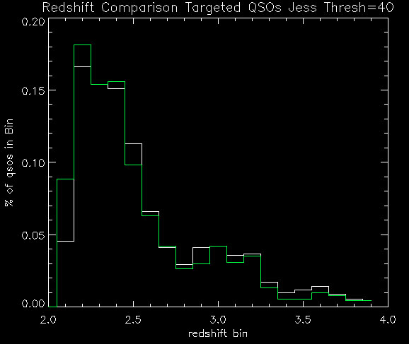
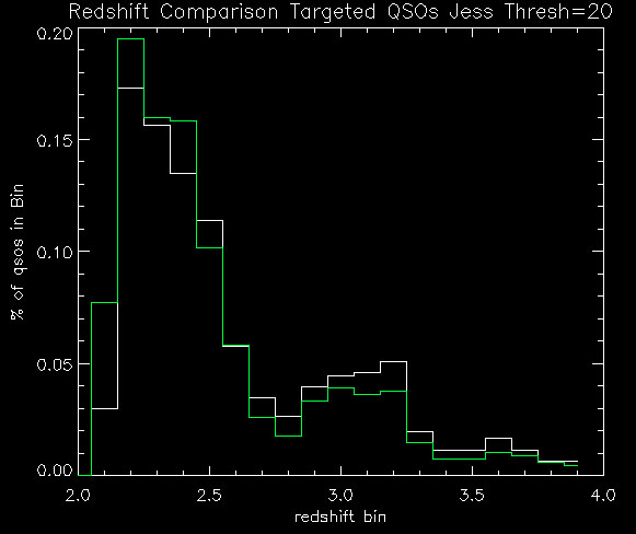
Below are plots (same as yesterday's post) + the likelihood ratio distributions. Again, white is v1 (old) and green is v2 (new):