One of the comments from Hennawi about my paper was he wanted to know how many unique quasars were simulated in the QSO catalog.
I wasn't exactly sure how to define "unique" quasar.
The simulated i-band fluxes range from 15 to 22.5. They are simulated to 4 decimal places.
The simulated redshifts (z) range from 0.5 to 5.0. They are simulated out to 6 decimal places.
If I define unique to be the same out to the maximum decimal places provided, then there are only 2 simulated quasars that are repeats of each other (0.00002%)
If I define unique to be within 0.1% magnitude/redshift of each other, then there are 6285 (out of 10 million) are repeats (0.06%).
If I define unique to be within 1% magnitude/redshift of each other, then there are 62,824 repeat objects (0.6%).
Anyway, so I guess I should ask Joe how he wants me to define repeats.
Here is the code to do this:
file = '/clusterfs/riemann/raid001/jessica/boss/Likeli_QSO.fits.gz'
qsos = mrdfits(file, 1)
imean = mean(qsos.i_sim)
zmean = mean(qsos.z_sim)
percent = 1.0/100. #simulated quasars within this percentage of each other
ierr = imean*percent
zerr = zmean*percent
imult = round(1./ierr)*1.
zmult = round(1./zerr)*1.
roundqsosz = round(qsos.z_sim*zmult)/zmult
roundqsosi = round(qsos.i_sim*zmult)/imult
uniqz = uniq(roundqsosz)
uniqi = uniq(roundqsosi)
all = where(qsos.z_sim GT -99999)
repeatZ = setdifference(all, uniqz)
repeatI = setdifference(all, uniqI)
help, setintersection(repeatZ, repeatI)
Also can be found in the following log file:
../logs/110313log.pro
Showing posts with label QSO Catalog. Show all posts
Showing posts with label QSO Catalog. Show all posts
Sunday, March 13, 2011
Tuesday, August 17, 2010
Overlapping Contours

;Turn on colors
device,true_color=24,decomposed=0,retain=2
;Set up fonts
!P.FONT = -1
!P.THICK = 1
DEVICE, SET_FONT ='Times Bold',/TT_FONT
white = GetColor('White', 1)
black = GetColor('Black', 2)
green = GetColor('Green', 3)
red = GetColor('Red', 4)
blue = GetColor('Blue',5)
LoadCT, 33, NColors=levels, Bottom=3
;Set up contour data
bin_width = 0.05
minx=-1.0
miny=-0.5
maxx=4
maxy=2
star_contours = HIST_2D(ugscolor, grscolor, bin1=bin_width, bin2=bin_width, max1=maxx, MAX2=maxy, MIN1=minx, MIN2=miny)
;; This sets up (max1-min1)bin1 bins in X....
x_cont = findgen(n_elements(star_contours[*,1]))
sx_cont = (x_cont*bin_width) + minx
;; And 60 bins in y
y_cont = findgen(n_elements(star_contours[1,*]))
sy_cont = (y_cont*bin_width) + miny
qso_contours = HIST_2D(ugqcolor, grqcolor, bin1=bin_width, bin2=bin_width, max1=maxx, MAX2=maxy, MIN1=minx, MIN2=miny)
;; This sets up (max1-min1)bin1 bins in X....
x_cont = findgen(n_elements(qso_contours[*,1]))
qx_cont = (x_cont*bin_width) + minx
;; And 60 bins in y
y_cont = findgen(n_elements(qso_contours[1,*]))
qy_cont = (y_cont*bin_width) + miny
levels = 10
userlevels = findgen(levels)^2.5
maxlevel = max(userlevels)
smax = max(star_contours)*1.1
slevels = userlevels*smax/maxlevel
levels = 7
userlevels = findgen(levels)^2.5
maxlevel = max(userlevels)
qmax = max(qso_contours)*1.1
qlevels = userlevels*qmax/maxlevel
mtitle = 'Color-Color Contour Plot'
xtitle = 'u-g magnitude'
ytitle = 'g-r magnitude'
Window, XSize=800, YSize=700
Contour, star_contours, sx_cont, sy_cont, C_Colors=red, Background=1, Levels=slevels, Color=black, XTITLE = xtitle, YTITLE = ytitle, TITLE = mtitle, charsize = 2, charthick = 1, thick=2, xthick=2, ythick=2
Contour, qso_contours, qx_cont, qy_cont, /Overplot, Levels=qLevels, Color=blue, thick=2
set_plot, 'ps'
!P.FONT = 0
!P.THICK = 1
aspect_ratio = (7.0/8.0)
xsz = 5.0
ysz = xsz*aspect_ratio
device, filename = 'contourqsostar.eps', /color, bits_per_pixel = 8,encapsul=0, xsize=xsz,ysize=ysz, /INCHES, /TIMES, /BOLD
Contour, star_contours, sx_cont, sy_cont, C_Colors=red, Background=1, Levels=slevels, Color=black, XTITLE = xtitle, YTITLE = ytitle, TITLE = mtitle, charsize = 1, charthick = 1, thick=2, xthick=2, ythick=2
Contour, qso_contours, qx_cont, qy_cont, /Overplot, Levels=qLevels, Color=blue, thick=2
device, /close
set_plot,'X'
!P.FONT = -1
!P.THICK = 1
DEVICE, SET_FONT ='Times Bold',/TT_FONT
log file:
../logs/100817log.pro
Monday, August 16, 2010
Final Plotting
From this page we see how to do color contour plots: http://www.dfanning.com/tips/contour_hole.html
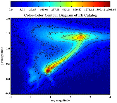
Here are the plots for the QSO and EE catalogs:
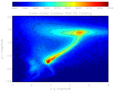
Here is the code to make them... I've used non-linear color levels to show peaks better...
For everything else catalog:
file1 = filepath('Likeli_everything.fits', root_dir=getenv('BOSSTARGET_DIR'), subdir='data')
;file1 = './Likeli_everything.fits.gz'
.com likelihood_compute
startemplate = likelihood_everything_file(file1, area=area1)
;Get magnitudes
;Star Magnitudes (don't need to deredden)
smag = 22.5 - 2.5*alog10(startemplate.psfflux>1.0d-3)
ugscolor = smag[0,*] - smag[1,*]
grscolor = smag[1,*] - smag[2,*]
;Turn on colors
device,true_color=24,decomposed=0,retain=2
;Set up fonts
!P.FONT = -1
!P.THICK = 1
DEVICE, SET_FONT ='Times Bold',/TT_FONT
bin_width = 0.025
minx=-1.0
miny=-0.5
maxx=4
maxy=2
;Create contours
star_contours = HIST_2D(ugscolor, grscolor, bin1=bin_width, bin2=bin_width, max1=maxx, MAX2=maxy, MIN1=minx, MIN2=miny)
;; This sets up (max1-min1)bin1 bins in X....
x_cont = findgen(n_elements(star_contours[*,1]))
x_cont = (x_cont*bin_width) + minx
;; And bins in y
y_cont = findgen(n_elements(star_contours[1,*]))
y_cont = (y_cont*bin_width) + miny
;Set up plot titles
xtitle = 'u-g magnitude'
ytitle = 'g-r magnitude'
mtitle = 'Color-Color Contour Plot EE Catalog'
levels = 256 ;plot in 256 colors
data = star_contours
x = x_cont
y = y_cont
white = GetColor('White', 1) ; know what is white
black = GetColor('Black', 2) ; know what is black
;load blue-red color table
LoadCT, 33, NColors=levels, Bottom=3
;define the levels of the color contours
;non linear to show data shape better
userlevels = findgen(levels)^3
maxlevel = max(userlevels)
thismax = max(star_contours)*1.1
userlevels = userlevels*thismax/maxlevel
;define the levels of the contour lines
;non linear to show data shape better
;only ten lines so that the text is legible
slevels = 10
suserlevels = findgen(slevels)^3
maxlevel = max(suserlevels)
thismax = max(star_contours)*1.1
suserlevels = suserlevels*thismax/maxlevel
; make window
Window, XSize=800, YSize=700
;Make contour plot
Contour, data, x, y, /Fill, C_Colors=Indgen(levels)+3, Background=1, Levels=userlevels, Position=[0.12, 0.1, 0.9, 0.80], Color=black, XTITLE = xtitle, YTITLE = ytitle, TITLE = mtitle, charsize = 2, charthick = 1, thick=1, xthick=2, ythick=2
;Overplot black lines
Contour, data, x, y, /Overplot, Levels=suserLevels, /Follow, Color=black
;Make color bar
ColorBar, NColors=levels, Bottom=3, Divisions=slevels-1, TICKNAMES=suserlevels, Range=[Min(data), Max(data)], Format='(G8.5)', Position = [0.12, 0.9, 0.9, 0.95], Color=black
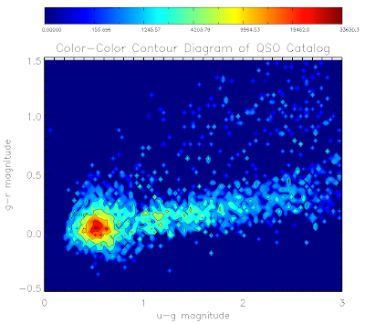
Similarly for the qso catalog:
bin_width = 0.03
minx=0.0
miny=-0.5
maxx=3.0
maxy=1.5
qso_contours = HIST_2D(ugqcolor, grqcolor, bin1=bin_width, bin2=bin_width, max1=maxx, MAX2=maxy, MIN1=minx, MIN2=miny)
;; This sets up (max1-min1)bin1 bins in X....
x_cont = findgen(n_elements(qso_contours[*,1]))
x_cont = (x_cont*bin_width) + minx
;; And 60 bins in y
y_cont = findgen(n_elements(qso_contours[1,*]))
y_cont = (y_cont*bin_width) + miny
xtitle = 'u-g magnitude'
ytitle = 'g-r magnitude'
mtitle = 'Color-Color Contour Diagram of QSO Catalog'
levels = 256
data = qso_contours
x = x_cont
y = y_cont
white = GetColor('White', 1)
black = GetColor('Black', 2)
LoadCT, 33, NColors=levels, Bottom=3
userlevels = findgen(levels)^3
maxlevel = max(userlevels)
thismax = max(qso_contours)*1.1
userlevels = userlevels*thismax/maxlevel
slevels = 7
suserlevels = findgen(slevels)^3
maxlevel = max(suserlevels)
thismax = max(qso_contours)*1.1
suserlevels = suserlevels*thismax/maxlevel
Window, XSize=800, YSize=700
Contour, data, x, y, /Fill, C_Colors=Indgen(levels)+3, Background=1, Levels=userlevels, Position=[0.12, 0.1, 0.9, 0.80], Color=black, XTITLE = xtitle, YTITLE = ytitle, TITLE = mtitle, charsize = 2, charthick = 1, thick=1, xthick=2, ythick=2
Contour, data, x, y, /Overplot, Levels=suserLevels, /Follow, Color=black
ColorBar, NColors=levels, Bottom=3, Divisions=slevels-1, TICKNAMES=suserlevels, Range=[Min(data), Max(data)], Format='(G10.5)', Position = [0.12, 0.9, 0.9, 0.95], Color=black
And to make the plots to files:
set_plot, 'ps'
!P.FONT = 0
!P.THICK = 1
aspect_ratio = (7.0/8.0)
xsz = 7.0
ysz = xsz*aspect_ratio
device, filename = 'contourstars.eps', /color, bits_per_pixel = 8,encapsul=0, xsize=xsz,ysize=ysz, /INCHES, /TIMES, /BOLD
Contour, data, x, y, /Fill, C_Colors=Indgen(levels)+3, Background=1, Levels=userlevels, Position=[0.11, 0.1, 0.9, 0.80], Color=black, XTITLE = xtitle, YTITLE = ytitle, TITLE = mtitle, charsize = 1, charthick = 1, thick=1, xthick=2, ythick=2
Contour, data, x, y, /Overplot, Levels=suserLevels, /Follow, Color=black
ColorBar, NColors=levels, Bottom=3, Divisions=slevels-1, TICKNAMES=suserlevels, Range=[Min(data), Max(data)], Format='(G8.5)', Position = [0.11, 0.9, 0.9, 0.95], Color=black
device, /close
set_plot,'X'
!P.FONT = -1
!P.THICK = 1
DEVICE, SET_FONT ='Times Bold',/TT_FONT
bin_width = 0.03
minx=0.0
miny=-0.5
maxx=3.0
maxy=1.5
qso_contours = HIST_2D(ugqcolor, grqcolor, bin1=bin_width, bin2=bin_width, max1=maxx, MAX2=maxy, MIN1=minx, MIN2=miny)
;; This sets up (max1-min1)bin1 bins in X....
x_cont = findgen(n_elements(qso_contours[*,1]))
x_cont = (x_cont*bin_width) + minx
;; And 60 bins in y
y_cont = findgen(n_elements(qso_contours[1,*]))
y_cont = (y_cont*bin_width) + miny
xtitle = 'u-g magnitude'
ytitle = 'g-r magnitude'
mtitle = 'Color-Color Contour Diagram of QSO Catalog'
levels = 256
data = qso_contours
x = x_cont
y = y_cont
white = GetColor('White', 1)
black = GetColor('Black', 2)
LoadCT, 33, NColors=levels, Bottom=3
userlevels = findgen(levels)^3
maxlevel = max(userlevels)
thismax = max(qso_contours)*1.1
userlevels = userlevels*thismax/maxlevel
slevels = 7
suserlevels = findgen(slevels)^3
maxlevel = max(suserlevels)
thismax = max(qso_contours)*1.1
suserlevels = suserlevels*thismax/maxlevel
set_plot, 'ps'
!P.FONT = 0
!P.THICK = 1
aspect_ratio = (7.0/8.0)
xsz = 7.0
ysz = xsz*aspect_ratio
device, filename = 'contourqsos.eps', /color, bits_per_pixel = 8,encapsul=0, xsize=xsz,ysize=ysz, /INCHES, /TIMES, /BOLD
Contour, data, x, y, /Fill, C_Colors=Indgen(levels)+3, Background=1, Levels=userlevels, Position=[0.12, 0.1, 0.9, 0.80], Color=black, XTITLE = xtitle, YTITLE = ytitle, TITLE = mtitle, charsize = 1, charthick = 1, thick=1, xthick=2, ythick=2
Contour, data, x, y, /Overplot, Levels=suserLevels, /Follow, Color=black
ColorBar, NColors=levels, Bottom=3, Divisions=slevels-1, TICKNAMES=suserlevels, Range=[Min(data), Max(data)], Format='(G10.5)', Position = [0.12, 0.9, 0.9, 0.95], Color=black
device, /close
set_plot,'X'
!P.FONT = -1
!P.THICK = 1
DEVICE, SET_FONT ='Times Bold',/TT_FONT
See they look pretty:
All in the following log file:
../logs/100816log.pro
Here are the plots for the QSO and EE catalogs:


Here is the code to make them... I've used non-linear color levels to show peaks better...
For everything else catalog:
file1 = filepath('Likeli_everything.fits', root_dir=getenv('BOSSTARGET_DIR'), subdir='data')
;file1 = './Likeli_everything.fits.gz'
.com likelihood_compute
startemplate = likelihood_everything_file(file1, area=area1)
;Get magnitudes
;Star Magnitudes (don't need to deredden)
smag = 22.5 - 2.5*alog10(startemplate.psfflux>1.0d-3)
ugscolor = smag[0,*] - smag[1,*]
grscolor = smag[1,*] - smag[2,*]
;Turn on colors
device,true_color=24,decomposed=0,retain=2
;Set up fonts
!P.FONT = -1
!P.THICK = 1
DEVICE, SET_FONT ='Times Bold',/TT_FONT
bin_width = 0.025
minx=-1.0
miny=-0.5
maxx=4
maxy=2
;Create contours
star_contours = HIST_2D(ugscolor, grscolor, bin1=bin_width, bin2=bin_width, max1=maxx, MAX2=maxy, MIN1=minx, MIN2=miny)
;; This sets up (max1-min1)bin1 bins in X....
x_cont = findgen(n_elements(star_contours[*,1]))
x_cont = (x_cont*bin_width) + minx
;; And bins in y
y_cont = findgen(n_elements(star_contours[1,*]))
y_cont = (y_cont*bin_width) + miny
;Set up plot titles
xtitle = 'u-g magnitude'
ytitle = 'g-r magnitude'
mtitle = 'Color-Color Contour Plot EE Catalog'
levels = 256 ;plot in 256 colors
data = star_contours
x = x_cont
y = y_cont
white = GetColor('White', 1) ; know what is white
black = GetColor('Black', 2) ; know what is black
;load blue-red color table
LoadCT, 33, NColors=levels, Bottom=3
;define the levels of the color contours
;non linear to show data shape better
userlevels = findgen(levels)^3
maxlevel = max(userlevels)
thismax = max(star_contours)*1.1
userlevels = userlevels*thismax/maxlevel
;define the levels of the contour lines
;non linear to show data shape better
;only ten lines so that the text is legible
slevels = 10
suserlevels = findgen(slevels)^3
maxlevel = max(suserlevels)
thismax = max(star_contours)*1.1
suserlevels = suserlevels*thismax/maxlevel
; make window
Window, XSize=800, YSize=700
;Make contour plot
Contour, data, x, y, /Fill, C_Colors=Indgen(levels)+3, Background=1, Levels=userlevels, Position=[0.12, 0.1, 0.9, 0.80], Color=black, XTITLE = xtitle, YTITLE = ytitle, TITLE = mtitle, charsize = 2, charthick = 1, thick=1, xthick=2, ythick=2
;Overplot black lines
Contour, data, x, y, /Overplot, Levels=suserLevels, /Follow, Color=black
;Make color bar
ColorBar, NColors=levels, Bottom=3, Divisions=slevels-1, TICKNAMES=suserlevels, Range=[Min(data), Max(data)], Format='(G8.5)', Position = [0.12, 0.9, 0.9, 0.95], Color=black
Similarly for the qso catalog:
bin_width = 0.03
minx=0.0
miny=-0.5
maxx=3.0
maxy=1.5
qso_contours = HIST_2D(ugqcolor, grqcolor, bin1=bin_width, bin2=bin_width, max1=maxx, MAX2=maxy, MIN1=minx, MIN2=miny)
;; This sets up (max1-min1)bin1 bins in X....
x_cont = findgen(n_elements(qso_contours[*,1]))
x_cont = (x_cont*bin_width) + minx
;; And 60 bins in y
y_cont = findgen(n_elements(qso_contours[1,*]))
y_cont = (y_cont*bin_width) + miny
xtitle = 'u-g magnitude'
ytitle = 'g-r magnitude'
mtitle = 'Color-Color Contour Diagram of QSO Catalog'
levels = 256
data = qso_contours
x = x_cont
y = y_cont
white = GetColor('White', 1)
black = GetColor('Black', 2)
LoadCT, 33, NColors=levels, Bottom=3
userlevels = findgen(levels)^3
maxlevel = max(userlevels)
thismax = max(qso_contours)*1.1
userlevels = userlevels*thismax/maxlevel
slevels = 7
suserlevels = findgen(slevels)^3
maxlevel = max(suserlevels)
thismax = max(qso_contours)*1.1
suserlevels = suserlevels*thismax/maxlevel
Window, XSize=800, YSize=700
Contour, data, x, y, /Fill, C_Colors=Indgen(levels)+3, Background=1, Levels=userlevels, Position=[0.12, 0.1, 0.9, 0.80], Color=black, XTITLE = xtitle, YTITLE = ytitle, TITLE = mtitle, charsize = 2, charthick = 1, thick=1, xthick=2, ythick=2
Contour, data, x, y, /Overplot, Levels=suserLevels, /Follow, Color=black
ColorBar, NColors=levels, Bottom=3, Divisions=slevels-1, TICKNAMES=suserlevels, Range=[Min(data), Max(data)], Format='(G10.5)', Position = [0.12, 0.9, 0.9, 0.95], Color=black
And to make the plots to files:
set_plot, 'ps'
!P.FONT = 0
!P.THICK = 1
aspect_ratio = (7.0/8.0)
xsz = 7.0
ysz = xsz*aspect_ratio
device, filename = 'contourstars.eps', /color, bits_per_pixel = 8,encapsul=0, xsize=xsz,ysize=ysz, /INCHES, /TIMES, /BOLD
Contour, data, x, y, /Fill, C_Colors=Indgen(levels)+3, Background=1, Levels=userlevels, Position=[0.11, 0.1, 0.9, 0.80], Color=black, XTITLE = xtitle, YTITLE = ytitle, TITLE = mtitle, charsize = 1, charthick = 1, thick=1, xthick=2, ythick=2
Contour, data, x, y, /Overplot, Levels=suserLevels, /Follow, Color=black
ColorBar, NColors=levels, Bottom=3, Divisions=slevels-1, TICKNAMES=suserlevels, Range=[Min(data), Max(data)], Format='(G8.5)', Position = [0.11, 0.9, 0.9, 0.95], Color=black
device, /close
set_plot,'X'
!P.FONT = -1
!P.THICK = 1
DEVICE, SET_FONT ='Times Bold',/TT_FONT
bin_width = 0.03
minx=0.0
miny=-0.5
maxx=3.0
maxy=1.5
qso_contours = HIST_2D(ugqcolor, grqcolor, bin1=bin_width, bin2=bin_width, max1=maxx, MAX2=maxy, MIN1=minx, MIN2=miny)
;; This sets up (max1-min1)bin1 bins in X....
x_cont = findgen(n_elements(qso_contours[*,1]))
x_cont = (x_cont*bin_width) + minx
;; And 60 bins in y
y_cont = findgen(n_elements(qso_contours[1,*]))
y_cont = (y_cont*bin_width) + miny
xtitle = 'u-g magnitude'
ytitle = 'g-r magnitude'
mtitle = 'Color-Color Contour Diagram of QSO Catalog'
levels = 256
data = qso_contours
x = x_cont
y = y_cont
white = GetColor('White', 1)
black = GetColor('Black', 2)
LoadCT, 33, NColors=levels, Bottom=3
userlevels = findgen(levels)^3
maxlevel = max(userlevels)
thismax = max(qso_contours)*1.1
userlevels = userlevels*thismax/maxlevel
slevels = 7
suserlevels = findgen(slevels)^3
maxlevel = max(suserlevels)
thismax = max(qso_contours)*1.1
suserlevels = suserlevels*thismax/maxlevel
set_plot, 'ps'
!P.FONT = 0
!P.THICK = 1
aspect_ratio = (7.0/8.0)
xsz = 7.0
ysz = xsz*aspect_ratio
device, filename = 'contourqsos.eps', /color, bits_per_pixel = 8,encapsul=0, xsize=xsz,ysize=ysz, /INCHES, /TIMES, /BOLD
Contour, data, x, y, /Fill, C_Colors=Indgen(levels)+3, Background=1, Levels=userlevels, Position=[0.12, 0.1, 0.9, 0.80], Color=black, XTITLE = xtitle, YTITLE = ytitle, TITLE = mtitle, charsize = 1, charthick = 1, thick=1, xthick=2, ythick=2
Contour, data, x, y, /Overplot, Levels=suserLevels, /Follow, Color=black
ColorBar, NColors=levels, Bottom=3, Divisions=slevels-1, TICKNAMES=suserlevels, Range=[Min(data), Max(data)], Format='(G10.5)', Position = [0.12, 0.9, 0.9, 0.95], Color=black
device, /close
set_plot,'X'
!P.FONT = -1
!P.THICK = 1
DEVICE, SET_FONT ='Times Bold',/TT_FONT
See they look pretty:


All in the following log file:
../logs/100816log.pro
Wednesday, May 12, 2010
ALL the Quasars
Recently Dinosaur Comics has been emphasizing ALL of everything. ALL the secrets, ALL the balls, ALL the burgers. So today we are going to creating the QSO catalog with ALL the Quasars.
Before we had a brightness limit and some other cuts, but Hennawi wanted me to see what it looked like with all of them.
I did this by modifying: qso_fake_jess.pro with the following call to qso_photosamp:
qsos = qso_photosamp(Z_MIN = Z_MIN, Z_MAX = Z_MAX, NOCUTS = NOCUTS, ILIM = 23.0)
Before we had a brightness limit and some other cuts, but Hennawi wanted me to see what it looked like with all of them.
I did this by modifying: qso_fake_jess.pro with the following call to qso_photosamp:
qsos = qso_photosamp(Z_MIN = Z_MIN, Z_MAX = Z_MAX, NOCUTS = NOCUTS, ILIM = 23.0)
Here is what these QSOs look like in color-color space:

And re-running hiz_kde_numerator_jess.pro:
.run hiz_kde_numerator_jess.pro
To create a new QSO Catalog:
../likelihood/qsocatalog/QSOCatalog-Wed-May-12-14:03:41-2010.fits
.run hiz_kde_numerator_jess.pro
To create a new QSO Catalog:
../likelihood/qsocatalog/QSOCatalog-Wed-May-12-14:03:41-2010.fits
Here is what the QSO Catalog looks like in color-color space:

Change likelihood_compute to read in this catalog:
; Read in the QSO file
file2 = '/home/jessica/repository/ccpzcalib/Jessica/likelihood/qsocatalog/QSOCatalog-Wed-May-12-14:03:41-2010.fits'
This run is in the directory:
../likelihood/likev1all
The log file is here:
../logs/100512log.pro
; Read in the QSO file
file2 = '/home/jessica/repository/ccpzcalib/Jessica/likelihood/qsocatalog/QSOCatalog-Wed-May-12-14:03:41-2010.fits'
This run is in the directory:
../likelihood/likev1all
The log file is here:
../logs/100512log.pro
~~~~~~~~
On a side note, I looked at Google Analytics for this blog today. It turns out that over it's lifetime 355 Absolute Unique vistors have viewed my blog! These visitors are from 10 countries and 28 different states. Pretty cool! Yet very few people leave comments on my blog. Everyone reading
this, leave a comment so I know you are out there!
this, leave a comment so I know you are out there!
~~~~~~~~
Is anyone else having problem's editing their blogspot blog using Google Chrome? It totally messes up the fonts and when I look at the html it is all funky. Seem strange considering google owns both Chrome and blogsplot! Maybe it is their way of punishing Mac users for the iPhone being better than the Google phone.
Tuesday, April 27, 2010
Likelihood Test Results (4)
Now I am going to see how the likelihood compares if we use the Richards luminosity function and we also include the (0.5 < z < 5.0). The code to run this is in the following log file: ../log/100427_3log.pro. This works even better than the last test:
eps = 1e-30
bossqsolike = total(likelihood.L_QSO_Z[16:32],1) ;quasars between redshift 2.1 and 3.7
qsolcut1 = where( alog10(total(likelihood.L_QSO_Z[16:32],1)) LT -9.0)
den = total(targets.L_EVERYTHING_ARRAY[0:4],1) + total(likelihood.L_QSO_Z[0:44],1) + eps
num = bossqsolike + eps
NEWRATIO = num/den
NEWRATIO[qsolcut1] = 0 ; eliminate objects with low L_QSO value
IDL> print, n_elements(ql) ; number quasars
461
IDL> print, n_elements(ql)*1.0/(n_elements(sl)+n_elements(ql)) ;percent accuracy
0.256111
IDL> print, n_elements(ql) + n_elements(sl) ; total targeted
1800
IDL>
IDL> print, n_elements(nql) ; number quasars
575
IDL> print, n_elements(nql)*1.0/(n_elements(nsl)+n_elements(nql)) ;percent accuracy
0.319444
IDL> print, n_elements(nql) + n_elements(nsl) ; total targeted
We now go from 25.6% accuracy to 31.9% accuracy! And we find 114 more quasars!
Plots
The white points were targeted/missed by both the new and old likelihoods
The magenta points were only targeted/missed by the new likelihood
The cyan points were only targeted/missed by the old likelihood


The white points were targeted/missed by both the new and old likelihoods
The magenta points were only targeted/missed by the new likelihood
The cyan points were only targeted/missed by the old likelihood


Monday, April 26, 2010
Likelihood Test Results (3)
As a sanity check I re-computed the likelihoods with the old qso catalog to make sure I got the same results as before, which I did. See ../logs/100426log.pro for code.
It seems that adding in the BOSS QSOs doesn't help.
Now I am going to run on the old qso catalog but with the larger redshift range (0.5 < z < 5.0) and see if this improves things. See ../logs/100426log.pro for code.
So this seems to actually make a difference. I have played around with the redshift range for the numerator to get the best selection numbers:
eps = 1e-30
bossqsolike = total(likelihood.L_QSO_Z[14:34],1) ;quasars between redshift 2.1 and 3.5
qsolcut1 = where( alog10(total(likelihood.L_QSO_Z[19:34],1)) LT -9.0)
den = total(targets.L_EVERYTHING_ARRAY[0:4],1) + total(likelihood.L_QSO_Z[0:44],1) + eps
num = bossqsolike + eps
NEWRATIO = num/den
NEWRATIO[qsolcut1] = 0 ; eliminate objects with low L_QSO value
qsolcut2 = where( alog10(total(targets.L_QSO_Z[0:18],1)) LT -9.0)
L_QSO = total(targets.L_QSO_Z[2:18],1)
den = total(targets.L_EVERYTHING_ARRAY[0:4],1) + total(targets.L_QSO_Z[0:18],1) + eps
num = L_QSO + eps
OLDRATIO = num/den
OLDRATIO[qsolcut2] = 0 ; eliminate objects with low L_QSO value
numsel = 1800-1
NRend = n_elements(newratio)-1
sortNR = reverse(sort(newratio))
targetNR = sortNR[0:numsel]
restNR = sortNR[numsel+1:NRend]
ORend = n_elements(oldratio)-1
sortOR = reverse(sort(oldratio))
targetOR = sortOR[0:numsel]
restOR = sortOR[numsel+1:ORend]
nql = setintersection(quasarindex,targetNR)
nqnl = setintersection(quasarindex, restNR)
nsl = setdifference(targetNR, quasarindex)
nsnl = setdifference(restNR, quasarindex)
ql = setintersection(quasarindex, targetOR)
qnl = setintersection(quasarindex, restOR)
sl = setdifference(targetOR,quasarindex)
snl = setdifference(restOR,quasarindex)
IDL> print, n_elements(ql) ; number quasars
461
IDL> print, n_elements(ql)*1.0/(n_elements(sl)+n_elements(ql)) ;percent accuracy
0.256111
IDL> print, n_elements(ql) + n_elements(sl) ; total targeted
1800
IDL>
IDL> print, n_elements(nql) ; number quasars
508
IDL> print, n_elements(nql)*1.0/(n_elements(nsl)+n_elements(nql)) ;percent accuracy
0.282222
IDL> print, n_elements(nql) + n_elements(nsl) ; total targeted
1800
So we go from 25.6% accuracy to 28.2% accuracy! And we find 47 more quasars!

The code for the above run is in the directory ../likelihood/run1/
Now to see how the different luminosity functions do. Below is results running with the Richard 06 luminosity function:

(See ../logs/100427_2log.pro for code)
IDL> print, n_elements(ql) ; number quasars
461
IDL> print, n_elements(ql)*1.0/(n_elements(sl)+n_elements(ql)) ;percent accuracy
0.256111
IDL> print, n_elements(ql) + n_elements(sl) ; total targeted
1800
IDL>
IDL> print, n_elements(nql) ; number quasars
543
IDL> print, n_elements(nql)*1.0/(n_elements(nsl)+n_elements(nql)) ;percent accuracy
0.301667
IDL> print, n_elements(nql) + n_elements(nsl) ; total targeted
1800
This does better than the old luminosity function!
So we go from 25.6% accuracy to 30.2% accuracy! And we find 82 more quasars!
It seems that adding in the BOSS QSOs doesn't help.
Now I am going to run on the old qso catalog but with the larger redshift range (0.5 < z < 5.0) and see if this improves things. See ../logs/100426log.pro for code.
So this seems to actually make a difference. I have played around with the redshift range for the numerator to get the best selection numbers:
eps = 1e-30
bossqsolike = total(likelihood.L_QSO_Z[14:34],1) ;quasars between redshift 2.1 and 3.5
qsolcut1 = where( alog10(total(likelihood.L_QSO_Z[19:34],1)) LT -9.0)
den = total(targets.L_EVERYTHING_ARRAY[0:4],1) + total(likelihood.L_QSO_Z[0:44],1) + eps
num = bossqsolike + eps
NEWRATIO = num/den
NEWRATIO[qsolcut1] = 0 ; eliminate objects with low L_QSO value
qsolcut2 = where( alog10(total(targets.L_QSO_Z[0:18],1)) LT -9.0)
L_QSO = total(targets.L_QSO_Z[2:18],1)
den = total(targets.L_EVERYTHING_ARRAY[0:4],1) + total(targets.L_QSO_Z[0:18],1) + eps
num = L_QSO + eps
OLDRATIO = num/den
OLDRATIO[qsolcut2] = 0 ; eliminate objects with low L_QSO value
numsel = 1800-1
NRend = n_elements(newratio)-1
sortNR = reverse(sort(newratio))
targetNR = sortNR[0:numsel]
restNR = sortNR[numsel+1:NRend]
ORend = n_elements(oldratio)-1
sortOR = reverse(sort(oldratio))
targetOR = sortOR[0:numsel]
restOR = sortOR[numsel+1:ORend]
nql = setintersection(quasarindex,targetNR)
nqnl = setintersection(quasarindex, restNR)
nsl = setdifference(targetNR, quasarindex)
nsnl = setdifference(restNR, quasarindex)
ql = setintersection(quasarindex, targetOR)
qnl = setintersection(quasarindex, restOR)
sl = setdifference(targetOR,quasarindex)
snl = setdifference(restOR,quasarindex)
IDL> print, n_elements(ql) ; number quasars
461
IDL> print, n_elements(ql)*1.0/(n_elements(sl)+n_elements(ql)) ;percent accuracy
0.256111
IDL> print, n_elements(ql) + n_elements(sl) ; total targeted
1800
IDL>
IDL> print, n_elements(nql) ; number quasars
508
IDL> print, n_elements(nql)*1.0/(n_elements(nsl)+n_elements(nql)) ;percent accuracy
0.282222
IDL> print, n_elements(nql) + n_elements(nsl) ; total targeted
1800
So we go from 25.6% accuracy to 28.2% accuracy! And we find 47 more quasars!
Plots
The white points were targeted/missed by both the new and old likelihoods
The magenta points were only targeted/missed by the new likelihood
The cyan points were only targeted/missed by the old likelihood

The white points were targeted/missed by both the new and old likelihoods
The magenta points were only targeted/missed by the new likelihood
The cyan points were only targeted/missed by the old likelihood


Now to see how the different luminosity functions do. Below is results running with the Richard 06 luminosity function:
QSO Catalog with Richards Luminosity Function

(See ../logs/100427_2log.pro for code)
IDL> print, n_elements(ql) ; number quasars
461
IDL> print, n_elements(ql)*1.0/(n_elements(sl)+n_elements(ql)) ;percent accuracy
0.256111
IDL> print, n_elements(ql) + n_elements(sl) ; total targeted
1800
IDL>
IDL> print, n_elements(nql) ; number quasars
543
IDL> print, n_elements(nql)*1.0/(n_elements(nsl)+n_elements(nql)) ;percent accuracy
0.301667
IDL> print, n_elements(nql) + n_elements(nsl) ; total targeted
1800
This does better than the old luminosity function!
So we go from 25.6% accuracy to 30.2% accuracy! And we find 82 more quasars!
Plots
The white points were targeted/missed by both the new and old likelihoods
The magenta points were only targeted/missed by the new likelihood
The cyan points were only targeted/missed by the old likelihood


The white points were targeted/missed by both the new and old likelihoods
The magenta points were only targeted/missed by the new likelihood
The cyan points were only targeted/missed by the old likelihood


Sunday, April 25, 2010
Likelihood Test Results (2)
I'm going to try adding in all QSOs (regardless of brightness). I've taken out the BOSS QSOs that are in Stripe-82 so that we don't have the same objects in the Monte Carlo as in the testing data.
Joe suggested doing this. We'll see if it improves things, if not, then looks like we should go back to old catalog and see if modifying the luminosity function helps.
Here is what they look like:


The code to do this is in the following log file: ../logs/100425log.pro
It creates the following file to use as input to Monte Carlo: ~/boss/allQSOMCInput.fits"

I re-ran hiz_kde_numerator_jess.pro to make a new QSOCatalog, which is here:
../likelihood/qsocatalog/QSOCatalog-Mon-Apr-26-13:22:43-2010.fits

I changed likelihood_compute to look at the above catalog.
Run the likelihood calculation with this new input catalog:
smalltargetfile = "./smalltarget.fits"
smalltargets = mrdfits(smalltargetfile, 1)
.com splittargets2.pro
nsplit = 50L
splitsize = floor(n_elements(smalltargets)*1.0/nsplit)
junk = splitTargets2(smalltargets, nsplit, splitsize)
; run likelihood.script
.com mergeLikelihoods.pro
likelihood = mergelikelihoods(nsplit)
outfile = "./likelihoods2.0-4.0ALLBOSSAddedSmall.fits"
splog, 'Writing file ', outfile
mwrfits, likelihood, outfile, /create
IDL> print, n_elements(ql) ; number quasars
467
IDL> print, n_elements(ql)*1.0/(n_elements(sl)+n_elements(ql)) ;percent accuracy
0.259300
IDL> print, n_elements(ql) + n_elements(sl) ; total targeted
1801
IDL>
IDL> print, n_elements(nql) ; number quasars
418
IDL> print, n_elements(nql)*1.0/(n_elements(nsl)+n_elements(nql)) ;percent accuracy
0.232093
IDL> print, n_elements(nql) + n_elements(nsl) ; total targeted
1801
This doesn't do better than the old likelihood either (same color scheme as last post).


The logfile for this is ../logs/100425log.pro
Joe suggested doing this. We'll see if it improves things, if not, then looks like we should go back to old catalog and see if modifying the luminosity function helps.
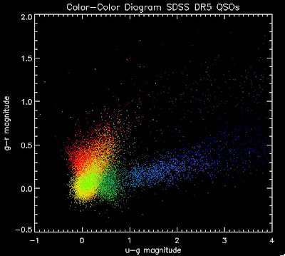
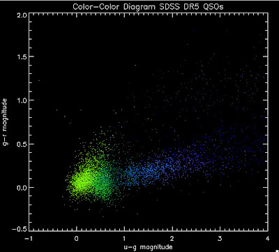
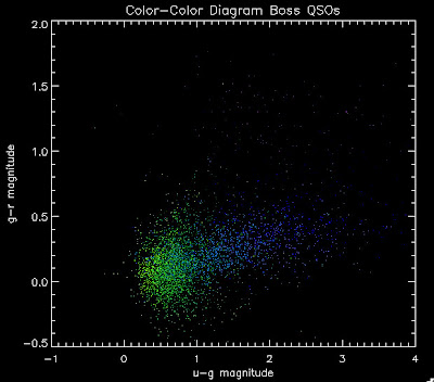
Here is what they look like:
BOSS QSOs

SDSS DR5 QSOs

The code to do this is in the following log file: ../logs/100425log.pro
It creates the following file to use as input to Monte Carlo: ~/boss/allQSOMCInput.fits"
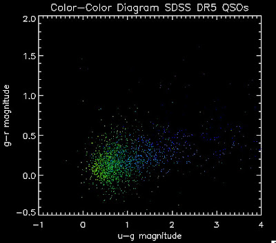
Plot of allQSOMCInput.fits

../likelihood/qsocatalog/QSOCatalog-Mon-Apr-26-13:22:43-2010.fits
Plot of QSOCatalog-Mon-Apr-26-13:22:43-2010.fits

I changed likelihood_compute to look at the above catalog.
Run the likelihood calculation with this new input catalog:
smalltargetfile = "./smalltarget.fits"
smalltargets = mrdfits(smalltargetfile, 1)
.com splittargets2.pro
nsplit = 50L
splitsize = floor(n_elements(smalltargets)*1.0/nsplit)
junk = splitTargets2(smalltargets, nsplit, splitsize)
; run likelihood.script
.com mergeLikelihoods.pro
likelihood = mergelikelihoods(nsplit)
outfile = "./likelihoods2.0-4.0ALLBOSSAddedSmall.fits"
splog, 'Writing file ', outfile
mwrfits, likelihood, outfile, /create
IDL> print, n_elements(ql) ; number quasars
467
IDL> print, n_elements(ql)*1.0/(n_elements(sl)+n_elements(ql)) ;percent accuracy
0.259300
IDL> print, n_elements(ql) + n_elements(sl) ; total targeted
1801
IDL>
IDL> print, n_elements(nql) ; number quasars
418
IDL> print, n_elements(nql)*1.0/(n_elements(nsl)+n_elements(nql)) ;percent accuracy
0.232093
IDL> print, n_elements(nql) + n_elements(nsl) ; total targeted
1801
This doesn't do better than the old likelihood either (same color scheme as last post).


The logfile for this is ../logs/100425log.pro
Wednesday, March 17, 2010
Changing QSO Catalog Inputs
I'm trying to figure out how to modify the inputs (currently SDSS DR5 quasars with good photometry) into Joe's Monte Carlo. Here is what I have figured out so far (all the below files are on riemann):
hiz_kde_numerator.pro ;main program to generate the QSO Catalog
(calls) →
qso_fakephoto.pro ;generates simulated redshift and i-magnitude based on luminosity function and DR5 inputs
(calls) →
qso_photosamp.pro ;This generates the training set photometry
(calls) →
sdss_read_data.pro ;This reads in SDSS data it currently has the following 'DR5' call
qsos = sdss_read_data('DR5', Z_MIN = Z_MIN, Z_MAX = Z_MAX)
Here is a color-color redshift temperature plot of these DR5 QSOs:
I'm going to try to add in the BOSS QSOs with co-added photometry, especially in the redshift range z > 2.0 where we seem to be missing QSOs:
I found that there are 1,973 BOSS quasars that have a redshift above 2.0 for which we also have coadded photometry. Here they are plotted:
While it is a little more filled in in the u-g = 0.8 space, comparing it to all the BOSS quasars (regardless of how good their photometry is) below:
hiz_kde_numerator.pro ;main program to generate the QSO Catalog
(calls) →
qso_fakephoto.pro ;generates simulated redshift and i-magnitude based on luminosity function and DR5 inputs
(calls) →
qso_photosamp.pro ;This generates the training set photometry
(calls) →
sdss_read_data.pro ;This reads in SDSS data it currently has the following 'DR5' call
qsos = sdss_read_data('DR5', Z_MIN = Z_MIN, Z_MAX = Z_MAX)
Here is a color-color redshift temperature plot of these DR5 QSOs:

I'm going to try to add in the BOSS QSOs with co-added photometry, especially in the redshift range z > 2.0 where we seem to be missing QSOs:

I found that there are 1,973 BOSS quasars that have a redshift above 2.0 for which we also have coadded photometry. Here they are plotted:

While it is a little more filled in in the u-g = 0.8 space, comparing it to all the BOSS quasars (regardless of how good their photometry is) below:

Tuesday, March 16, 2010
Comparing Quasars
Here are the color-color diagrams with redshift temperature plots for the current QSO Catalog (in the BOSS redshift range) and the BOSS 3PC Quasars (same temperature-z map as before). I think this shows pretty well that something is wrong with the QSO Catalog's color distribution. These both have the same number of quasars, in the same redshift range:

Their redshift distributions are not that different so this is really a matter of the input QSOs not properly representing the spread of the possible colors, I believe:
 White is BOSS QSOs, Green is the QSO Catalog.
The histograms are scaled as a percentage in each bin.
I want to add in BOSS QSOs to Joe's Monte Carlo. We can do this by just adding in the "chunk 1" objects where we have co-added photometry from Stripe-82, or we can apply the same cuts in terms of brightness as we did to the DR5 catalog.
Friday, March 12, 2010
Plots for Joe (and Brandon)
Aside - A couple weeks ago Brandon Basso complained that my buzzing wasn't frequent enough. He requested more plots and perhaps an update on Adam's research. Well ask and you shall receive! Brandon this plot-heavy post is dedicated to you.
I am trying to understand why we seem to be missing objects around u-g = 0.8. Joe suggested I make the color plots in different redshift bins. So here we go. Warning, there are a lot of plots.
First, let me show you a temperature plots of the different luminosity functions. Below are color-color diagrams where the color of the points changes as a function of redshift in the following way:
dark red = 1.0 < z < 1.2
red = 1.2 < z < 1.4
orange red = 1.4 < z < 1.6
orange = 1.6 < z < 1.8
gold = 1.8 < z < 2.0
lawn green = 2.0 < z < 2.2
lime green =2.2 < z < 2.4
dark green = 2.4 < z < 2.6
teal = 2.6 < z < 2.8
dodger blue = 2.8 < z < 3.0
royal blue = 3.0 < z < 3.2
blue = 3.2 < z < 3.4
navy= 3.4 < z < 3.6
dark slate blue = 3.6 < z < 3.8
dark orchid = 3.8 < z < 4.0
As a reminder here are the luminosity functions I am using:
 The above plot shows several luminosity functions.
Green is Richards 06, cyan is Jiang, purple is Jiang Combined (what we used in previous QSO Catalog, white is a Richard/Jiang average (suggested by Myers).
Here are the color-color redshift temperature plots for the QSO Catalogs generated by the above luminosity functions (click plots on below to make larger):


Also I have made color-color plots binned by redshift separately. I've done them for all of the luminosity functions, but they all look pretty much the same, so I'll just post them here for the Richards function (green luminosity function above), the redshift range is in the main title of the plots:


Here are some histograms of various quantities for the different luminosity functions the color scheme is same as above, Green is Richards 06, cyan is Jiang, purple is Jiang Combined (what we used in previous QSO Catalog, white is a Richard/Jiang average:
redshift

Color-band psffluxes


Color-band magnitudes


Color-band magnitudes


Color-color plot u-g/g-r


Hopefully that is enough plots for Joe to see what is going on with these QSO catalogs and Brandon to be satisfied.
Oh and here is an update on Adam's research (check out his shirt).
Subscribe to:
Posts (Atom)
