Tuesday, March 30, 2010
1M Reconstruction (Take Two)
I've started running on a larger data set. I'm trying to re-run the 1M reconstruction from before to see if I can get a better reconstruction with the fixed the 2D correlation function. Results to follow once the run is done, but the working directory is: .../pythonJess/run2010330_178
Monday, March 29, 2010
Data Run
I'm running the reconstruction on the data. I'm doing in the working directory: .../pythonJess/run2010329_1319. I am running this with 12 redshift bins and 250k photometric and spectroscopic objects.
I did a little bit of thinking about the number of grids for the correlation function. There is the strange balance that you want the number of grids to be less than the number of particles, otherwise you might as well just correlate all possible pairs. You also want the spacing to be much bigger than the max correlation length, otherwise even by going out one grid length, you will unnecessarily correlate too many objects. I feel like this is a computer science problem, and perhaps Adam Pauls or Erin Sheldon would know the answer?
I played with this a bit (tried upping the grid points to 1000, and this took forever to run). For the 2D correlation function, I am correlating out to a distance of 0.34 (with a box size of 1). Maybe I don't need to correlate out to such a big angle? We could probably have as few as 10 grid points in each dimension if we are going out to this large of an angle. For the 3D correlation function, I am correlating out to a distance of 20 Mpc/h (with a box size of 2400 Mpc/h) so we need at least ~120 grid points in each dimension.
For the 3D correlation function, some of the larger redshift bins have very few objects in them, and if we have ~1003 or 106 grid points then we are wasting time griding if we have less than 103 points in each set.
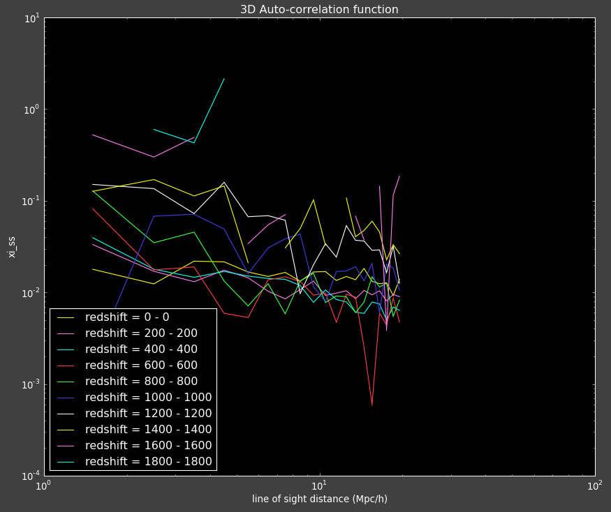
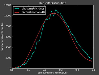
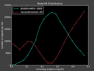
Here are the results from the reconstruction I ran yesterday. It looks like I don't have enough points because the correlation functions are very noisy.


The reconstructions don't look good and are highly variable:


I did a little bit of thinking about the number of grids for the correlation function. There is the strange balance that you want the number of grids to be less than the number of particles, otherwise you might as well just correlate all possible pairs. You also want the spacing to be much bigger than the max correlation length, otherwise even by going out one grid length, you will unnecessarily correlate too many objects. I feel like this is a computer science problem, and perhaps Adam Pauls or Erin Sheldon would know the answer?
I played with this a bit (tried upping the grid points to 1000, and this took forever to run). For the 2D correlation function, I am correlating out to a distance of 0.34 (with a box size of 1). Maybe I don't need to correlate out to such a big angle? We could probably have as few as 10 grid points in each dimension if we are going out to this large of an angle. For the 3D correlation function, I am correlating out to a distance of 20 Mpc/h (with a box size of 2400 Mpc/h) so we need at least ~120 grid points in each dimension.
For the 3D correlation function, some of the larger redshift bins have very few objects in them, and if we have ~1003 or 106 grid points then we are wasting time griding if we have less than 103 points in each set.
Here are the results from the reconstruction I ran yesterday. It looks like I don't have enough points because the correlation functions are very noisy.

The reconstructions don't look good and are highly variable:


I'm running on a bigger data set now.
Friday, March 26, 2010
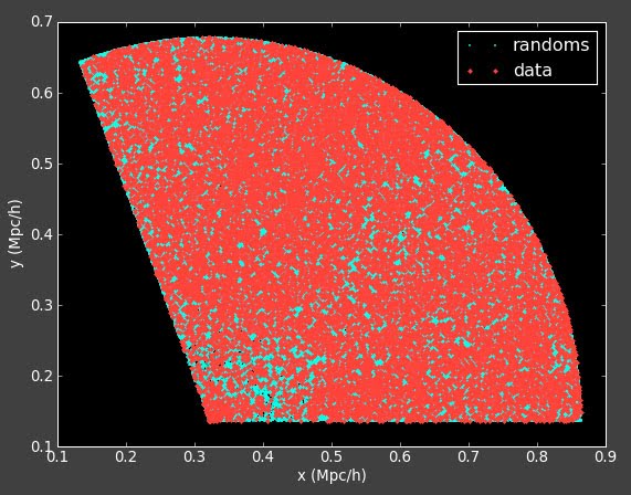
Mask Fixed
It turns out that my mask was messing up. I now have it fixed. Here is what the data/randoms look like on the mock data:


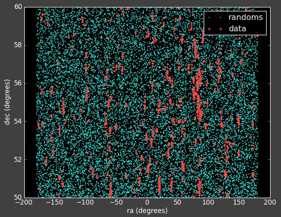


And here is what is looks like for real data:


The log on 3/29 has the code to run these.


The log on 3/29 has the code to run these.
Wednesday, March 24, 2010
If It Isn't One Correlation Function, It's Another!
I ran my code on the Stripe-82 data for the first time since I fixed the angular correlation functions and now my 3D correlation functions look weird:

I think this has something to do with some changes I made to the conversion from ra/dec to x, y, z. I had been doing something that I don't think is right before and I changed that, but it might now be messing up the masks so that my mask for the 3D correlation functions are now not in the same region as the data. I'm going back to look at the changes I made to investigate this. Thank goodness for repositories!
Tuesday, March 23, 2010
Playing with crl
I'm trying to fix the binning issues I was having with the reconstruction. Alexia suggested playing with the crl file.
In her email on March 10, subject: improving cross-correlation , she says:
"Go to the part of getCoeff in the crl.py file. There are two choices for for the matrix B (for a flat prior and for a linear prior). Comment out the linear and uncomment the flat, and rerun to see if you get the same behavior for a particular binning choice, or if you get the same TYPE of behavior with the new B, but not correlated to the specific bin choice."
I did above and here are some plots (left is with a constant prior and right is with linear prior):

Currently:
if tol > 0
lam*=10
else:
lam/=10


if lambda is 100:
Flat prior


if lambda is 1:
Linear prior


In her email on March 10, subject: improving cross-corr
"Go to the part of getCoeff in the crl.py file. There are two choices for for the matrix B (for a flat prior and for a linear prior). Comment out the linear and uncomment the flat, and rerun to see if you get the same behavior for a particular binning choice, or if you get the same TYPE of behavior with the new B, but not correlated to the specific bin choice."
I did above and here are some plots (left is with a constant prior and right is with linear prior):


This doesn't seem to change things much. I talked to Alexia on the phone today and she also suggested I change the value of lambda to see how that effects things.
Currently:
if tol > 0
lam*=10
else:
lam/=10
I'm looking at what changing these numbers (lambda) does to the reconstruction...
if lambda is 5:
Flat prior


Linear prior


if lambda is 100:
Flat prior


Linear Prior:


if lambda is 1:
Linear prior


Flat prior


Alexia doesn't think I should worry to much about this right now, but I thought I'd make some plots for her to look and think about.
On the to do list:
Run reconstruction on real data
Check the mesh to see if this is the cause of the correlation function taking so long to compute.
On the to do list:
Run reconstruction on real data
Check the mesh to see if this is the cause of the correlation function taking so long to compute.
Wednesday, March 17, 2010
Changing QSO Catalog Inputs
I'm trying to figure out how to modify the inputs (currently SDSS DR5 quasars with good photometry) into Joe's Monte Carlo. Here is what I have figured out so far (all the below files are on riemann):
hiz_kde_numerator.pro ;main program to generate the QSO Catalog
(calls) →
qso_fakephoto.pro ;generates simulated redshift and i-magnitude based on luminosity function and DR5 inputs
(calls) →
qso_photosamp.pro ;This generates the training set photometry
(calls) →
sdss_read_data.pro ;This reads in SDSS data it currently has the following 'DR5' call
qsos = sdss_read_data('DR5', Z_MIN = Z_MIN, Z_MAX = Z_MAX)
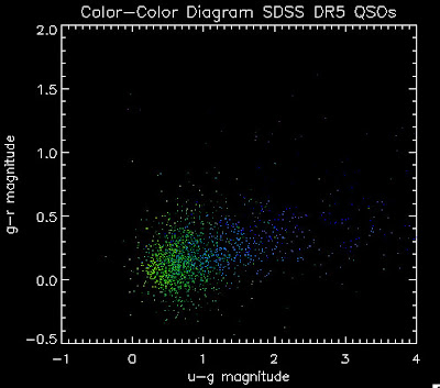
Here is a color-color redshift temperature plot of these DR5 QSOs:
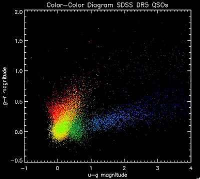
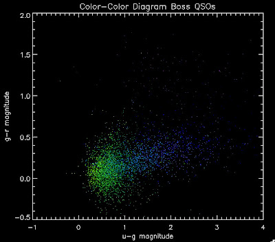
I'm going to try to add in the BOSS QSOs with co-added photometry, especially in the redshift range z > 2.0 where we seem to be missing QSOs:
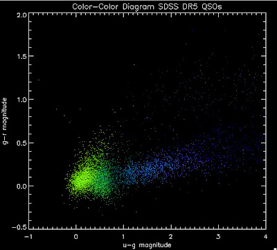
I found that there are 1,973 BOSS quasars that have a redshift above 2.0 for which we also have coadded photometry. Here they are plotted:
While it is a little more filled in in the u-g = 0.8 space, comparing it to all the BOSS quasars (regardless of how good their photometry is) below:
hiz_kde_numerator.pro ;main program to generate the QSO Catalog
(calls) →
qso_fakephoto.pro ;generates simulated redshift and i-magnitude based on luminosity function and DR5 inputs
(calls) →
qso_photosamp.pro ;This generates the training set photometry
(calls) →
sdss_read_data.pro ;This reads in SDSS data it currently has the following 'DR5' call
qsos = sdss_read_data('DR5', Z_MIN = Z_MIN, Z_MAX = Z_MAX)
Here is a color-color redshift temperature plot of these DR5 QSOs:

I'm going to try to add in the BOSS QSOs with co-added photometry, especially in the redshift range z > 2.0 where we seem to be missing QSOs:

I found that there are 1,973 BOSS quasars that have a redshift above 2.0 for which we also have coadded photometry. Here they are plotted:

While it is a little more filled in in the u-g = 0.8 space, comparing it to all the BOSS quasars (regardless of how good their photometry is) below:

Tuesday, March 16, 2010
Comparing Quasars
Here are the color-color diagrams with redshift temperature plots for the current QSO Catalog (in the BOSS redshift range) and the BOSS 3PC Quasars (same temperature-z map as before). I think this shows pretty well that something is wrong with the QSO Catalog's color distribution. These both have the same number of quasars, in the same redshift range:

Their redshift distributions are not that different so this is really a matter of the input QSOs not properly representing the spread of the possible colors, I believe:
 White is BOSS QSOs, Green is the QSO Catalog.
The histograms are scaled as a percentage in each bin.
I want to add in BOSS QSOs to Joe's Monte Carlo. We can do this by just adding in the "chunk 1" objects where we have co-added photometry from Stripe-82, or we can apply the same cuts in terms of brightness as we did to the DR5 catalog.
Monday, March 15, 2010
Useful IDL Commands
I need to do some work for the likelihood project and thus code in IDL again. Because I am not working in IDL very frequently, I tend to forgot commands and syntax. I thought it would be useful to compile a list of commands here so that I don't have to keep looking these up again and again.
number of elements in an array:
print, N_ELEMENTS(array)
unix command in idl: dollar sign ($) before command
$pwd
$ls
list all variables currently being used:
help
doc_library, 'spherematch' -- man page for the function
which, 'spherematch' --- tells you where in the IDL path the function is.
when recompiling idlutils need to use evilmake
!pi is constant pi
plothist (makes histogram plot)
when looking at a structure you use the /str command:
help, mystructure, /str
reading a fits file using mrdfits:
filedata = mrdfits(file2read, 1)
Combine two structures of the same size:
struct3 =struct_combine(struct1,struct2)
Concatenate two structure of the same type:
struct3 = [struct1, struct2]
Plotting Histogram (from here):
total with higher precision: total(...., /double)
in for loops:
for j = 0L, rsize-1 do begin
the L makes j a long int.
;Show color table
colorName = PickColorName(startColorName)
; Make heat map (warning, not very sophisticated)
colorobject = qsotemplate1.z_sim
xobject = ugqcolor1
yobject = grqcolor1
colorbin = 0.3
colorstart = 1.0
colorstop = colorstart + colorbin
plot, xobject[0:1], yobject[0:1], ps=null, color=fsc_color('white'), xr=[-0.5,4],yr=[-0.5,2], XTITLE = 'u-g magnitude', YTITLE = 'g-r magnitude', TITLE = 'Color-Color Diagram QSO Catalog Jiang Combo', charsize = 1.5, charthick = 1
zrange = where(colorobject GE colorstart AND colorobject LT colorstop)
oplot, xobject[zrange], yobject[zrange], ps=3, color=FSC_COLOR('dark red') ;Fake QSOs
colorstart = colorstop
colorstop = colorstart + colorbin
zrange = where(colorobject GE colorstart AND colorobject LT colorstop)
oplot, xobject[zrange], yobject[zrange], ps=3, color=FSC_COLOR('red') ;Fake QSOs
colorstart = colorstop
colorstop = colorstart + colorbin
zrange = where(colorobject GE colorstart AND colorobject LT colorstop)
oplot, xobject[zrange], yobject[zrange], ps=3, color=FSC_COLOR('orange red') ;Fake QSOs
colorstart = colorstop
colorstop = colorstart + colorbin
zrange = where(colorobject GE colorstart AND colorobject LT colorstop)
oplot, xobject[zrange], yobject[zrange], ps=3, color=FSC_COLOR('orange') ;Fake QSO
colorstart = colorstop
colorstop = colorstart + colorbin
zrange = where(colorobject GE colorstart AND colorobject LT colorstop)
oplot, xobject[zrange], yobject[zrange], ps=3, color=FSC_COLOR('gold') ;Fake QSOs
colorstart = colorstop
colorstop = colorstart + colorbin
zrange = where(colorobject GE colorstart AND colorobject LT colorstop)
oplot, xobject[zrange], yobject[zrange], ps=3, color=FSC_COLOR('lawn green') ;Fake QSOs
colorstart = colorstop
colorstop = colorstart + colorbin
zrange = where(colorobject GE colorstart AND colorobject LT colorstop)
oplot, xobject[zrange], yobject[zrange], ps=3, color=FSC_COLOR('lime green') ;Fake QSOs
colorstart = colorstop
colorstop = colorstart + colorbin
zrange = where(colorobject GE colorstart AND colorobject LT colorstop)
oplot, xobject[zrange], yobject[zrange], ps=3, color=FSC_COLOR('dark green') ;Fake QSOs
colorstart = colorstop
colorstop = colorstart + colorbin
zrange = where(colorobject GE colorstart AND colorobject LT colorstop)
oplot, xobject[zrange], yobject[zrange], ps=3, color=FSC_COLOR('teal') ;Fake QSOs
colorstart = colorstop
colorstop = colorstart + colorbin
zrange = where(colorobject GE colorstart AND colorobject LT colorstop)
oplot, xobject[zrange], yobject[zrange], ps=3, color=FSC_COLOR('dodger blue') ;Fake QSOs
colorstart = colorstop
colorstop = colorstart + colorbin
zrange = where(colorobject GE colorstart AND colorobject LT colorstop)
oplot, xobject[zrange], yobject[zrange], ps=3, color=FSC_COLOR('royal blue') ;Fake QSOs
colorstart = colorstop
colorstop = colorstart + colorbin
zrange = where(colorobject GE colorstart AND colorobject LT colorstop)
oplot, xobject[zrange], yobject[zrange], ps=3, color=FSC_COLOR('blue') ;Fake QSOs
colorstart = colorstop
colorstop = colorstart + colorbin
zrange = where(colorobject GE colorstart AND colorobject LT colorstop)
oplot, xobject[zrange], yobject[zrange], ps=3, color=FSC_COLOR('navy') ;Fake QSOs
colorstart = colorstop
colorstop = colorstart + colorbin
zrange = where(colorobject GE colorstart AND colorobject LT colorstop)
oplot, xobject[zrange], yobject[zrange], ps=3, color=FSC_COLOR('dark slate blue') ;Fake QSOs
colorstart = colorstop
colorstop = colorstart + colorbin
zrange = where(colorobject GE colorstart AND colorobject LT colorstop)
oplot, xobject[zrange], yobject[zrange], ps=3, color=FSC_COLOR('dark orchid') ;Fake QSOs
number of elements in an array:
print, N_ELEMENTS(array)
unix command in idl: dollar sign ($) before command
$pwd
$ls
list all variables currently being used:
help
doc_library, 'spherematch' -- man page for the function
which, 'spherematch' --- tells you where in the IDL path the function is.
when recompiling idlutils need to use evilmake
!pi is constant pi
plothist (makes histogram plot)
when looking at a structure you use the /str command:
help, mystructure, /str
reading a fits file using mrdfits:
filedata = mrdfits(file2read, 1)
Combine two structures of the same size:
struct3 =struct_combine(struct1,struct2)
Concatenate two structure of the same type:
struct3 = [struct1, struct2]
Plotting Histogram (from here):
PRO t_histogramIf you add maxmatch=1 to your spherematch it will avoid duplicates (should default to this)
data = [[-5, 4, 2, -8, 1], $
[ 3, 0, 5, -5, 1], $
[ 6, -7, 4, -4, -8], $
[-1, -5, -14, 2, 1]]
hist = HISTOGRAM(data)
bins = FINDGEN(N_ELEMENTS(hist)) + MIN(data)
PRINT, MIN(hist)
PRINT, bins
SPLOT, bins, hist, YRANGE = [MIN(hist)-1, MAX(hist)+1], PSYM = 10, XTITLE = 'Bin Number', YTITLE = 'Density per Bin'
END
total with higher precision: total(...., /double)
in for loops:
for j = 0L, rsize-1 do begin
the L makes j a long int.
;Show color table
colorName = PickColorName(startColorName)

; Make heat map (warning, not very sophisticated)

colorobject = qsotemplate1.z_sim
xobject = ugqcolor1
yobject = grqcolor1
colorbin = 0.3
colorstart = 1.0
colorstop = colorstart + colorbin
plot, xobject[0:1], yobject[0:1], ps=null, color=fsc_color('white'), xr=[-0.5,4],yr=[-0.5,2], XTITLE = 'u-g magnitude', YTITLE = 'g-r magnitude', TITLE = 'Color-Color Diagram QSO Catalog Jiang Combo', charsize = 1.5, charthick = 1
zrange = where(colorobject GE colorstart AND colorobject LT colorstop)
oplot, xobject[zrange], yobject[zrange], ps=3, color=FSC_COLOR('dark red') ;Fake QSOs
colorstart = colorstop
colorstop = colorstart + colorbin
zrange = where(colorobject GE colorstart AND colorobject LT colorstop)
oplot, xobject[zrange], yobject[zrange], ps=3, color=FSC_COLOR('red') ;Fake QSOs
colorstart = colorstop
colorstop = colorstart + colorbin
zrange = where(colorobject GE colorstart AND colorobject LT colorstop)
oplot, xobject[zrange], yobject[zrange], ps=3, color=FSC_COLOR('orange red') ;Fake QSOs
colorstart = colorstop
colorstop = colorstart + colorbin
zrange = where(colorobject GE colorstart AND colorobject LT colorstop)
oplot, xobject[zrange], yobject[zrange], ps=3, color=FSC_COLOR('orange') ;Fake QSO
colorstart = colorstop
colorstop = colorstart + colorbin
zrange = where(colorobject GE colorstart AND colorobject LT colorstop)
oplot, xobject[zrange], yobject[zrange], ps=3, color=FSC_COLOR('gold') ;Fake QSOs
colorstart = colorstop
colorstop = colorstart + colorbin
zrange = where(colorobject GE colorstart AND colorobject LT colorstop)
oplot, xobject[zrange], yobject[zrange], ps=3, color=FSC_COLOR('lawn green') ;Fake QSOs
colorstart = colorstop
colorstop = colorstart + colorbin
zrange = where(colorobject GE colorstart AND colorobject LT colorstop)
oplot, xobject[zrange], yobject[zrange], ps=3, color=FSC_COLOR('lime green') ;Fake QSOs
colorstart = colorstop
colorstop = colorstart + colorbin
zrange = where(colorobject GE colorstart AND colorobject LT colorstop)
oplot, xobject[zrange], yobject[zrange], ps=3, color=FSC_COLOR('dark green') ;Fake QSOs
colorstart = colorstop
colorstop = colorstart + colorbin
zrange = where(colorobject GE colorstart AND colorobject LT colorstop)
oplot, xobject[zrange], yobject[zrange], ps=3, color=FSC_COLOR('teal') ;Fake QSOs
colorstart = colorstop
colorstop = colorstart + colorbin
zrange = where(colorobject GE colorstart AND colorobject LT colorstop)
oplot, xobject[zrange], yobject[zrange], ps=3, color=FSC_COLOR('dodger blue') ;Fake QSOs
colorstart = colorstop
colorstop = colorstart + colorbin
zrange = where(colorobject GE colorstart AND colorobject LT colorstop)
oplot, xobject[zrange], yobject[zrange], ps=3, color=FSC_COLOR('royal blue') ;Fake QSOs
colorstart = colorstop
colorstop = colorstart + colorbin
zrange = where(colorobject GE colorstart AND colorobject LT colorstop)
oplot, xobject[zrange], yobject[zrange], ps=3, color=FSC_COLOR('blue') ;Fake QSOs
colorstart = colorstop
colorstop = colorstart + colorbin
zrange = where(colorobject GE colorstart AND colorobject LT colorstop)
oplot, xobject[zrange], yobject[zrange], ps=3, color=FSC_COLOR('navy') ;Fake QSOs
colorstart = colorstop
colorstop = colorstart + colorbin
zrange = where(colorobject GE colorstart AND colorobject LT colorstop)
oplot, xobject[zrange], yobject[zrange], ps=3, color=FSC_COLOR('dark slate blue') ;Fake QSOs
colorstart = colorstop
colorstop = colorstart + colorbin
zrange = where(colorobject GE colorstart AND colorobject LT colorstop)
oplot, xobject[zrange], yobject[zrange], ps=3, color=FSC_COLOR('dark orchid') ;Fake QSOs
The hope is that I will expand on this list every time I come across something I think I might use again (but don't use enough to memorize).
Friday, March 12, 2010
Plots for Joe (and Brandon)
Aside - A couple weeks ago Brandon Basso complained that my buzzing wasn't frequent enough. He requested more plots and perhaps an update on Adam's research. Well ask and you shall receive! Brandon this plot-heavy post is dedicated to you.
I am trying to understand why we seem to be missing objects around u-g = 0.8. Joe suggested I make the color plots in different redshift bins. So here we go. Warning, there are a lot of plots.
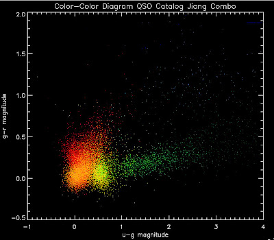
First, let me show you a temperature plots of the different luminosity functions. Below are color-color diagrams where the color of the points changes as a function of redshift in the following way:
I am trying to understand why we seem to be missing objects around u-g = 0.8. Joe suggested I make the color plots in different redshift bins. So here we go. Warning, there are a lot of plots.
First, let me show you a temperature plots of the different luminosity functions. Below are color-color diagrams where the color of the points changes as a function of redshift in the following way:
dark red = 1.0 < z < 1.2
red = 1.2 < z < 1.4
orange red = 1.4 < z < 1.6
orange = 1.6 < z < 1.8
gold = 1.8 < z < 2.0
lawn green = 2.0 < z < 2.2
lime green =2.2 < z < 2.4
dark green = 2.4 < z < 2.6
teal = 2.6 < z < 2.8
dodger blue = 2.8 < z < 3.0
royal blue = 3.0 < z < 3.2
blue = 3.2 < z < 3.4
navy= 3.4 < z < 3.6
dark slate blue = 3.6 < z < 3.8
dark orchid = 3.8 < z < 4.0
As a reminder here are the luminosity functions I am using:
 The above plot shows several luminosity functions.
Green is Richards 06, cyan is Jiang, purple is Jiang Combined (what we used in previous QSO Catalog, white is a Richard/Jiang average (suggested by Myers).
Here are the color-color redshift temperature plots for the QSO Catalogs generated by the above luminosity functions (click plots on below to make larger):


Also I have made color-color plots binned by redshift separately. I've done them for all of the luminosity functions, but they all look pretty much the same, so I'll just post them here for the Richards function (green luminosity function above), the redshift range is in the main title of the plots:


Here are some histograms of various quantities for the different luminosity functions the color scheme is same as above, Green is Richards 06, cyan is Jiang, purple is Jiang Combined (what we used in previous QSO Catalog, white is a Richard/Jiang average:
redshift

Color-band psffluxes


Color-band magnitudes


Color-band magnitudes


Color-color plot u-g/g-r


Hopefully that is enough plots for Joe to see what is going on with these QSO catalogs and Brandon to be satisfied.
Oh and here is an update on Adam's research (check out his shirt).
Subscribe to:
Posts (Atom)
