So Far So Good...

I have been working on systematically changing my 2D correlation function (which matches Alexia's 2d correlation function) to a 3D correlation function (which was looking very different from Alexia's 3D). I haven't made all the changes, but of those I have made thus far, I still get matching functions:

I haven't put in the coordinate changes yet (which is the major change, and probably the root of my problem). Let this experience be a reminder to me that I shouldn't make multiple changes at once to my code.

If you are wondering why this plot of Alexia's Xi looks different than the one in the Miserable Failure post, this is because that 3D correlation function was using an older version of Alexia's code which only looks at the correlation function in a cone with a 12 degree open angle. This version of her code calculates the correlation function on the entire box.

Time for the 'State of the Department' address. Predicted summary: We are broke!

Bad Hard Variables

Apologies for the lack of posting. It is just embarrassing to post day after day "still trying to find the error in my code." I am tempted to switch back to working on the likelihood stuff because at least I might have some progress to report. However, Josh tells me that if I don't post on my blog he is forced to do his own research -- I can't disappoint my readers (all two of them).

It turns out that there were some hard-wired constants in Alexia's 2D correlation function that I forgot about. When I adjusted those for the mock catalog I got my 2D function to match hers (thank goodness something is working):

Next step is to systematically make the changes from the 2D to the 3D until it breaks. I hate debugging.

Oh, and I can't believe how much nicer it has to have a software CRYPTOcard. Thank you Josh for helping me get one!

Still in Failure Mode

I've gone through and re-checked the conversions in my 3D-autocorrelation code to make sure I wasn't making any silly mistakes there. I couldn't find anything

I then decided I would go back to where I know the code is working (my 3D-autocorrelation code is a modification of some 2D (angular) correlation code). The 2D correlation code is comparable to some well-tested code that Alexia has (because it is in the same geometry) and I have in the past run these codes on the same files and gotten the same result. I ran my 2D code and Alexia's 2D code on Martin White's mock file, and I get the following 2D angular correlation functions (wps):

For some reason these aren't matching anymore even though they do match when I run it on a file of Sloan Data:

The plot thickens da da doom....

Traveling

I am traveling and will not be posting today.

Miserable Failure

Thank you to Kevin Young for finding some errors in my coordinate change code (now fixed).

I ran my correlation code on the mock data set. Here is my 3D auto-correlation function compared with Alexia's:

There is obviously something wrong with my correlation function. My correlation function isn't completely featureless:

I need to debug this, but not at 5pm on a Friday.

HTML Tip of the Day:
If you want text to have the exact formating (in terms of white space) that you type into the HTML then you can surround it with this <PRE> </PRE> tag pair and it will look like it did when you typed it. This is useful for keeping the correct formatting in my python code when I post it here.
http://www.maproom.co.uk/invis1.htm

Comma versus Plus

It turns out there was a bug in my coordinate change code:
mockR = N.sqrt(mockX**2 + mockY**2, mockZ**2)
when I should have had:
mockR = N.sqrt(mockX**2 + mockY**2 + mockZ**2)

Why it didn't come up with an error when there was a comma there, I don't know! Regardless, now I get the following when I plot the original z versus the converted back z:

And now I have written some lovely python functions to do these conversions for me in the future:

def xyz2thetaPhiR(thisx,thisy,thisz):
     radial = N.sqrt(thisx**2 + thisy**2 + thisz**2)
     polar = N.sqrt(thisx**2 + thisy**2)
     theta = N.arctan2(polar, thisz)
     phi = N.arctan2(thisy, thisx)
     return [theta,phi,radial]

def thetaPhiR2XYZ(theta,phi,radial):
     thisx = radial*N.cos(phi)*N.sin(theta)
     thisy = radial*N.sin(phi)*N.sin(theta)
     thisz = radial*N.cos(theta)
     return [thisx,thisy,thisz]

Now to run the correlation function on these ra/dec coordinates...

Coordinate Confusion

Time to run my 3D autocorrelation function on a mock catalog where we know the answer to try to see if there is a problem with my code or that the reconstruction is failing for another reason. I downloaded the following raw mock LRG catalog from Martin White's web page: halo_000_0.8000.dat.gz. I discovered that I can transfer files to riemann via the insure replacement by doing a two step scp. That is useful to know.

The code I am using to convert from ra, dec (degrees), comoving distance (r) to x, y, z and back:

%  x=r*sin(pi/2-pi/180*dec)*cos(pi/180*ra);
%  y=r*sin(pi/2-pi/180*dec)*sin(pi/180*ra);
%  z=r*cos(pi/2-pi/180*dec) ;

%  r = sqrt(x^2 + y^2 + z^2)
%  dec =  90 - 180/pi*arccos(z/r)
%  ra = 180/pi*arcsin(y/sqrt(x^2 + y^2))

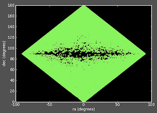
I am a little confused because these mock files are in Cartesian coordinates and if I convert them using the above code into ra and dec, I don't get the objects populating all of ra/dec space:

I constrained the data to be in a sphere of radius 0.5 boxsize (936.0 Mpc/h), and I would think that the ra and dec would then go from 0 to 360 and 0 to 180 respectively.

After some digging, I discovered that by using the arctan2 function I get the proper range:

%  theta = arctan2(sqrt(x^2+y^2), z)
%  phi = arctan2(x, y)

However when I try to then convert back to Cartesian I get a strange answer when I plot the original z versus the converted back z:

This is distressing!

Sources:
http://astro.uchicago.edu/cosmus/tech/code/radecz2xxyyzz.m
http://www.atlasoftheuniverse.com/cosmodis.c
http://www.math.montana.edu/frankw/ccp/multiworld/multipleIVP/spherical/body.htm
http://www.daniweb.com/forums/post860497-2.html

Python tips for the day
1) If you are getting the following error when trying to plot:

RuntimeError: Agg rendering complexity exceeded.
Consider downsampling or decimating your data

Then exit and restart your session and try again and it for some reason works. Stupid python.

2) When converting from spherical use atan2 not asin.

Traveling

I am traveling and will not be posting for the next few days.

I am HUGE in Berkeley (and NY)

Blogger.com was down last Thursday and not allowing me to post. Sorry for all of you who were eagerly awaiting my blog postings and disappointed by me not fulfilling my quota last week. Apparently my not posting (combined with not returning phone calls) made my father think I had died. Sorry Dad!

Below is the belated post for Thursday:
I re-ran the 3D auto-correlation function code with courser binning as suggested by Alexia. My result is not that different, although I did figure out how to put axes labels and a legend on my plots, so all was not lost!



The numbers in the legend represent the lower edge of the line-of-sight bin of the spectroscopic data in the 3D auto-correlation function in Mpc. So for instance the yellow line is a bin from 0-200 Mpc, the redline is from 600-800 Mpc etc.

I installed Google Analytics on this blog. Apparently my fan base is mostly Berkeley (5 visits -- probably mostly myself?) followed by New York (3 visits -- Demetri? Kathryn?). Unfortunately no visits from Princeton which means Alexia isn't reading this. Ha ha, busted!

Next step is to try calculating the 3D correlation function on a fake data set and comparing it to the known answer to make sure this isn't a bug in my code.

Tools of the Trade

I've found some useful tools for blog writing when you are trying to insert equations and images.

• On-line LaTeX Equation Editor makes pretty equations for you.
• HTML Help Page gives me the HTML for all the greek letters I need to use.
• Grab Application for Mac OS X allows me to get plots from a remote computer easily
• Adobe Photoshop allows me to invert said plots so they look pretty on my black-background blog.

~~~~~

I talked with Eric Gawiser today. He has thought a bit about the Newman method and had some good suggestions for me. He suggested that we would expect bias to be a function of redshift in the Sloan data set, and therefore we would have trouble properly normalizing our reconstruction because it would be the actual redshift distribution convolved with the bias function. He said that perhaps we could get a handle on the bias as a function of redshift by doing a 3D-autocorrelation function on the photometric data. I am not sure if this is already taken into account with the reconstruction or if the reconstruction is assuming a constant bias over redshift bins. This is something I need to talk to Alexia about. Nonetheless, Eric seems to know a lot about this and would be a good person to keep talking to about it.

~~~~~

I talked to David about the SVM-Light package. He seemed not so enthused. He said he wanted me to work out some other problems before I moved on to "code optimization." We went over how they ended up doing the selection on the QSOs using the likelihood method. He wants me to work out the normalization of the likelihood function so that the numbers actually mean something logical. He also isn't convinced that the MMT data is actually what we think it is. Apparently the method was only 75% complete with a 40% efficiency, so that isn't good. He wants me to get to the bottom of this and see if the QSO objects in the MMT data are actually quasars by comparing with Robert daSilva's variability catalogues. He also wants to check how good the method works on single-epoch data (they were running it on the co-added photometry).

He suggested that perhaps I run Michael Blanton's photo-z code on the Stripe-82 co-adds and use that at my data set for the Newman project. He suspects the photo-z's will be better than the single epoch data. He also suggested that perhaps a reason why my 3D correlation functions look so weird is because we get fiber collisions which wipe out correlations and ~Mpc scales (depending on redshift). Another reason to perhaps try this on mock data before I debug for years trying to find an error in my code (it's possible this method just wont work on this data set).

~~~~~

I gave the link to this blog to Alexia, and posted it on Facebook. I am fulfilling the whole "being accountable to people" rule. I guess I should change the blog's privacy settings so it is Google-able [DONE], and perhaps should add a link to my webpage. I hate the idea of people actually reading this (not that I think I am that important).

Deconstruction

The basic idea of the Newman Method redshift distribution reconstruction code is to take two sets of data which overlap in sky position (ra, dec). One set (let's call it S) is spectroscopic data where we have known redshifts. The other set (P) is photometric data where we do not know the redshifts (or at least don't know them very accurately). Next, I bin S into line of sight (los) distance bins. In the example I am describing here I have binned S from 200 Mpc/h to 1400 Mpc/h with a bin width of 200 Mpc/h. Then we take the angular correlation function, ω(los,θ), [see Landy, Szalay (1993) and Masjedi et al. (2006) for definitions of correlation functions] between each of these binned subsets of S and P. We then take the 3D auto-correlation, ξ(r) of the binned S with itself. The redshift distribution, φ, of P can be reconstructed by inverting the following sum over N bins:

ref: Schulz and White in Prep.

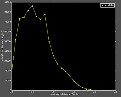
I am applying this method to galaxies in the Sloan data set. Here is what I expect the reconstructed redshift distribution to be (based on the photo-z's of the photometric data):

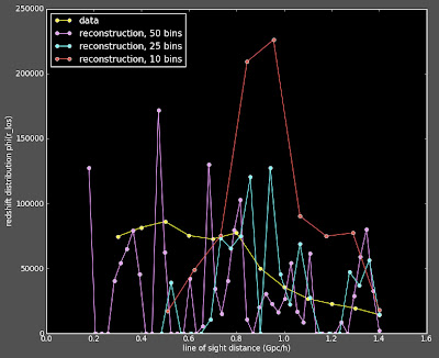
However when I run the reconstruction code, I get answers which do not look anything like this redshift distribution. More disturbing is that I get answer which vary wildly depending on how many φ bins I use in the reconstruction (which makes no sense at all to me). See below plot:

Alexia thinks that perhaps there is something wrong with my 3D-correlation function (it looks pretty featureless and smooth). So the next step is to try different binning of ξ(r) to see if perhaps this allows for better reconstruction -- maybe I am using too many bins and this is causing problems because the correlation function doesn't work properly if it doesn't have enough objects to reconstruct? David suggested that I try running my code on a set of mock data where we know the answer (and we've gotten the code to work before on this data). This will help me separate out if this is a issue with my version of the code, with the data (I am using photometric data and pretending that the photo-z's are the actual redshifts, which may not be good enough), or with the Newman method itself.

Lost in Translation

I've been having this problem that when I run my 3D auto-correlation function code on my laptop it runs fine, and gives me a logical result, but when I run the same code on my LBNL machine (riemann, for those who are familiar) I get a Segmentation fault and the code crashes. The code has the same inputs for both machines. The scarier thing is that when I run the code on a file with more data points, it doesn't crash on either machine.

However, I'm supposed to write about research accomplishments, so let me show the autocorrelation functions of the files that DID run:

3D auto-correlation function

2D cross-correlation function

I think the problem is that the files which are crashing have so few data points that there are some correlation bins where there are no objects separated by that distance. I am not actually sure how the code handles this. I would hope that it would just set that bin to zero, but there is quite likely a divide by zero problem going on here. Time to insert some print statements and get to the root of this.

A Light Idea

I have been talking to Adam Pauls about this likelihood method for selecting quasars for BOSS in SDSS-III. He has suggested looking into this application: SVM-Light. SVM is a support vector machine. It is basically a well-establish classification system for multivariate systems. The interesting thing about this program is that I can not only use it to optimize the likelihood algorithm, but I can put in the results of other classification algorithms (we are also using neural net and KDE methods) and use those as additional "variables" in my system. I could also use additional information like sky position or photometric redshift to add weights to different objects. Adam is showing me how to use this, and I am hoping it will be useful for optimizing the selection codes.

A Likely Result

In SDSS-III, the BOSS project is targeting 160,000 quasars (QSOs) at redshifts between 2.2 and 3.5. A color-color plot of spectroscopically confirmed QSOs (green) and stars (red). You can see that the quasars and stars have regions of overlap in the color space, and are therefore difficult to distinguish from each other.

David Schlegel suggested using a likelihood estimator to select quasars from stars. The basic idea is to have a templates of "quasar objects" and "all other objects" we would expect to see in the Sloan data set. We then take a "test object," one which we are trying to determine if it is a quasar or not, and compute a likelihood between it and the two templates. The likelihood of a test object (i) is for a set of template data (j) with color filters (f) is defined as follows:

where x is the flux of an object in the template data and mu is the flux of your test object and sigma if the error in your test object flux measurement.

I computed this likelihood with a set of test object where I knew if they were quasars or not. Below is a plot of the above likelihood computed on the test objects with a "quasar template" and a "everything else template." I am plotting the likelihood of the test objects with everything else (on the x axis) versus with quasars (on the y axis). Because I know what these test objects are, I can color the quasars (green) and the stars (blue). You can see that I get a clear separation in likelihood-likelihood space of these populations, where the quasars fall along a higher likelihood for quasars and the stars fall along a higher likelihood for everything else: