Cloudcroft Talk

Comparing Correlation Functions

I've been trying to figure out why my 2d Correlation Functions look weird. I've put out request to several Berkeley folks to compare my correlation function results on a data set with theirs, but while I wait for them to respond, I'm going to compare to some literature.

For the 2-d angular correlation function on SDSS LRG galaxies, I have the following plots from Connolly et al (2001):



And from Ross et al (2007):


I changed the angular bins of my correlation function to match these sets to try to form a comparison. Here is my 2D correlation function on BOSS data:

As you can see the slope of the function is much shallower for my correlation function, than it is the literature.

The 3D correlation functions are a better match:
From Ross et al (2007):

And here is mine:

At least the slopes seem to be comparable.

I am currently running the 3D correlation function on a larger los range to try to compare to Kazin et al. :

This will take a bit because I am correlating out to such large scales (180 Mpc/h).

Another thing I noticed that I wanted to talk to Alexia about is the actual computation of the correlation function in the code. Right now it is the following:

xi = (dd - dr - rd + rr)/rr

where

dd = # of data-data pairs in bin
dr = (# if data-random pairs in bin) / (Random Oversampling)
rd = (# if data-random pairs in bin) / (Random Oversampling)
rr = (# if random-random pairs in bin) / (Random Oversampling)

I am wondering if the rr should be divided by (random oversampling)^2 because there are that many more point in the RR set. I haven't changed this code from when I first got it from Alexia, so I assume it is correct. But I was looking the Landy, Szalay Paper and it seemed like they were using factors of n(n-1)/2 which is approximately n^2, and we are using factors of n.

Thoughts?

3/21 5:15 Update: Here is my plot of the 3d Correlation function on the large los range, it looks very similar to the Kazin plot above, you can even see the BAO signal @ ~100 Mpc/h:

Likelihood Paper

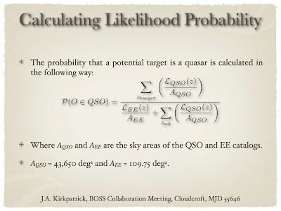
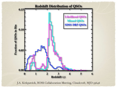
SDSS-III Publication 33: A Simple Likelihood Estimator for Quasar Target Selection

Authors: Jessica A. Kirkpatrick (corresponding author)
David J. Schlegel, Nicholas P. Ross, Adam D. Myers, Joseph F. Hennawi

Abstract:
We present a new method for quasar target selection using a likelihood estimator. For our purposes we target quasars using Sloan Digital Sky Survey (SDSS) photometry to a magnitude limit of g=22. The efficiency and completeness of this technique is measured using Baryon Oscillation Spectroscopic Survey (BOSS) Commissioning Data, taken in late 2009. This technique was used as the CORE method for target selection for BOSS Year 1 spectroscopy to be realized in the 9th SDSS data release (DR9). When targeting at a density of 40 objects/deg² we find the efficiency of this technique to be 41% and the completeness compared to all quasars identified in BOSS Commissioning Data to be 62%. This paper also describes possible extensions and improvements for this technique.

Comments:
SDSS-III participants have three weeks to send comments and to request changes. Participants comments should be sent to the Jessica Kirkpatrick.
The deadline to submit comments is Wednesday, April 6th 2011.

This is a BOSS science paper intended for submission to the Astrophysical Journal.

Downloads:
The most up to date .pdf of the paper can be found here:
likelihood paper (current) this version will be updated as I receive comments during the next three weeks.

The version of the paper submitted to the collaboration (3/16) is here:
likelihood collaboration submission

There is also a single column, double spaced version here (for easier editing):
likelihood paper one column

The .tex files and all associated figures, can be checked-out from the SVN at this location:
svn co svn+ssh://sdss3svn@sdss3.org/repo/boss/bosstarget/trunk/tex/likelihood/

Or downloaded here on the SDSS3 wiki.

Unique Quasars

One of the comments from Hennawi about my paper was he wanted to know how many unique quasars were simulated in the QSO catalog.

I wasn't exactly sure how to define "unique" quasar.

The simulated i-band fluxes range from 15 to 22.5. They are simulated to 4 decimal places.
The simulated redshifts (z) range from 0.5 to 5.0. They are simulated out to 6 decimal places.

If I define unique to be the same out to the maximum decimal places provided, then there are only 2 simulated quasars that are repeats of each other (0.00002%)

If I define unique to be within 0.1% magnitude/redshift of each other, then there are 6285 (out of 10 million) are repeats (0.06%).

If I define unique to be within 1% magnitude/redshift of each other, then there are 62,824 repeat objects (0.6%).

Anyway, so I guess I should ask Joe how he wants me to define repeats.

Here is the code to do this:
file = '/clusterfs/riemann/raid001/jessica/boss/Likeli_QSO.fits.gz'
qsos = mrdfits(file, 1)

imean = mean(qsos.i_sim)
zmean = mean(qsos.z_sim)

percent = 1.0/100. #simulated quasars within this percentage of each other
ierr = imean*percent
zerr = zmean*percent

imult = round(1./ierr)*1.
zmult = round(1./zerr)*1.

roundqsosz = round(qsos.z_sim*zmult)/zmult
roundqsosi = round(qsos.i_sim*zmult)/imult

uniqz = uniq(roundqsosz)
uniqi = uniq(roundqsosi)

all = where(qsos.z_sim GT -99999)

repeatZ = setdifference(all, uniqz)
repeatI = setdifference(all, uniqI)

help, setintersection(repeatZ, repeatI)

Also can be found in the following log file:
../logs/110313log.pro

About BOSS Data from Percival

Got word from Will Percival over the weekend:
He said the mask for the data/randoms is here:

https://trac.sdss3.org/browser/repo/boss/bosslss/trunk/geometry/current_boss_geometry.ply

He said:
I used the current_boss_geometry, choosing sectors with > 70% completeness. I don't have this separately in a file I'm afraid, but you could easily create it by placing the random catalog within the current_boss_geometry file - taking the quoted numbers as the completeness.

I said:
Thanks for the response. In terms of the 'current_boss_geometry' file. Is this as old as the randoms/galaxy files? Because I could imagine a scenario where the geometry file covers MORE area than the data files (because more of the sky has been observed) and then when I apply this "mask" to my other data it would let in regions of the sky which are not in the BOSS data files.

He said:
The current_boss_geometry file will always cover a larger area than that of the galaxies observed with completeness > 70%. But you can only use those polygons that contain one of the randoms. This will cut it back.

I said:
Also, how are you dealing with the spectroscopic completeness when generating the randoms? Are you basically filtering for each sky polygon based on the completeness in the current_boss_geometry file? For instance if a polygon has 80% completeness, then only 80% of randoms generated in that polygon are kept?

He said:
Yes, this is what I'm doing, based on the number of observed galaxies over the number of targets.

Using the BOSS Randoms

I downloaded the latest BOSS data and randoms from Will Percival as Martin White suggested in my email exchange with him yesterday.

There are in the following location on the wiki:
https://trac.sdss3.org/wiki/BOSS/clustering/cats

I put them here on riemann:

/clusterfs/riemann/raid001/jessica/boss/
galaxy-wjp-main008-LOWZ-020211-cut.txt
random-wjp-main008-LOWZ-020211-cut-small.txt
galaxy-wjp-merge-CMASS-020211-cut.txt
random-wjp-merge-CMASS-020211-cut-small.txt

The format of these files is:
ra / degrees
dec / degrees
redshift
galaxy weight
sector completeness
close pair flag
THING_ID
MASK POLY ID
ID for galaxy in spAll file (not in std format)

I read them in and below are plots. As you can see, the distribution of the randoms matches the data. So there is something wrong with what I am doing. At this point though, I'm not going to waste more time trying to fix my masks/randoms. I'm going to use these catalogs and re-run the correlation functions to see if this fixes things.

I'm also going to ask Shirley or Eric to run a correlation function on the same data to check that we get the same answer.



The code to make the above plots is in the following log file:
../logs/110302log/pro


thisfile = '/clusterfs/riemann/raid001/jessica/boss/galaxy-wjp-main008-LOWZ-020211-cut.txt'
readcol,thisfile,slra,sldec,slz,x,x,x,x,x,x,format='(F,F,F,F,F,F,F,F,F)'

thisfile = '/clusterfs/riemann/raid001/jessica/boss/galaxy-wjp-merge-CMASS-020211-cut.txt'
readcol,thisfile,sra,sdec,sz,x,x,x,x,x,x,format='(F,F,F,F,F,F,F,F,F)'

sra = [sra,slra]
sdec = [sdec,sldec]
sz = [sz,slz]



thisfile = '/clusterfs/riemann/raid001/jessica/boss/random-wjp-main008-LOWZ-020211-cut-small.txt'
readcol,thisfile,rslra,rsldec,rslz,x,x,x,x,x,x,format='(F,F,F,F,F,F,F,F,F)'

thisfile = '/clusterfs/riemann/raid001/jessica/boss/random-wjp-merge-CMASS-020211-cut-small.txt'
readcol,thisfile,rsra,rsdec,rsz,x,x,x,x,x,x,format='(F,F,F,F,F,F,F,F,F)'

rsra = [rsra,rslra]
rsdec = [rsdec,rsldec]
rsz = [rsz,rslz]



xtit = 'Ra'
ytit = 'Dec'
mtit = 'Ra vs Dec'
window,xsize=700,ysize=600
plot, sra, sdec, ps = 3, xrange = [110,130], yrange=[40,55],XTITLE = xtit, YTITLE =ytit, TITLE = mtit, charsize = 1.5, charthick = 1
oplot, rsra, rsdec, ps=3, color = fsc_color('green')



;Make histogram of the dec distributions
data = sdec
datamin = min(sdec)
datamax = max(sdec)
binsize = (datamax - datamin)/100
xtit = 'Dec Distribution'
ytit = '% in bin'
mtit = 'Histogram of Spectroscopic Dec'

window,xsize=700,ysize=600
hist = HISTOGRAM(data, binsize = binsize, min = datamin, max = datamax)
bins = FINDGEN(N_ELEMENTS(hist))*binsize + datamin
plot, bins, hist*1.0/n_elements(data), PSYM = 10, xrange = [datamin,datamax], yrange=[0,1.0*max(hist)/n_elements(data)],XTITLE = xtit, YTITLE =ytit, TITLE = mtit, charsize = 1.5, charthick = 1

data = rsdec
datamin = min(rsdec)
datamax = max(rsdec)
hist = HISTOGRAM(data, binsize = binsize, min = datamin, max = datamax)
bins = FINDGEN(N_ELEMENTS(hist))*binsize + datamin
oplot, bins, 1.0*hist/n_elements(data), PSYM = 10, color = fsc_color('green')



;Make histogram of the dec distributions
data = sdec
datamin = min(sdec)
datamax = max(sdec)
binsize = (datamax - datamin)/1000
xtit = 'Dec Distribution'
ytit = '# in bin'
mtit = 'Histogram of Spectroscopic Dec'

window,xsize=700,ysize=600
hist = HISTOGRAM(data, binsize = binsize, min = datamin, max = datamax)
bins = FINDGEN(N_ELEMENTS(hist))*binsize + datamin
plot, bins, hist*1.0, PSYM = 10, xrange = [datamin,datamax], yrange=[0,1.0*max(hist)],XTITLE = xtit, YTITLE =ytit, TITLE = mtit, charsize = 1.5, charthick = 1

data = rsdec
datamin = min(rsdec)
datamax = max(rsdec)
hist = HISTOGRAM(data, binsize = binsize, min = datamin, max = datamax)
bins = FINDGEN(N_ELEMENTS(hist))*binsize + datamin
oplot, bins, 1.0*hist, PSYM = 10, color = fsc_color('green')




;Make histogram of the dec distributions
data = sra
datamin = min(sra)
datamax = max(sra)
binsize = (datamax - datamin)/100
xtit = 'Ra Distribution'
ytit = '% in bin'
mtit = 'Histogram of Spectroscopic Ra'

window,xsize=700,ysize=600
hist = HISTOGRAM(data, binsize = binsize, min = datamin, max = datamax)
bins = FINDGEN(N_ELEMENTS(hist))*binsize + datamin
plot, bins, hist*1.0/n_elements(data), PSYM = 10, xrange = [datamin,datamax], yrange=[0,1.0*max(hist)/n_elements(data)],XTITLE = xtit, YTITLE =ytit, TITLE = mtit, charsize = 1.5, charthick = 1

data = rsra
datamin = min(rsra)
datamax = max(rsra)
hist = HISTOGRAM(data, binsize = binsize, min = datamin, max = datamax)
bins = FINDGEN(N_ELEMENTS(hist))*binsize + datamin
oplot, bins, 1.0*hist/n_elements(data), PSYM = 10, color = fsc_color('green')



;Make histogram of the dec distributions
data = sra
datamin = min(sra)
datamax = max(sra)
binsize = (datamax - datamin)/1000
xtit = 'RA Distribution'
ytit = '# in bin'
mtit = 'Histogram of Spectroscopic RA'

window,xsize=700,ysize=600
hist = HISTOGRAM(data, binsize = binsize, min = datamin, max = datamax)
bins = FINDGEN(N_ELEMENTS(hist))*binsize + datamin
plot, bins, hist*1.0, PSYM = 10, xrange = [datamin,datamax], yrange=[0,1.0*max(hist)],XTITLE = xtit, YTITLE =ytit, TITLE = mtit, charsize = 1.5, charthick = 1

data = rsra
datamin = min(rsra)
datamax = max(rsra)
hist = HISTOGRAM(data, binsize = binsize, min = datamin, max = datamax)
bins = FINDGEN(N_ELEMENTS(hist))*binsize + datamin
oplot, bins, 1.0*hist, PSYM = 10, color = fsc_color('green')



;Make histogram of the z distributions
data = sz
datamin = min(sz)
datamax = max(sz)
binsize = (datamax - datamin)/50
xtit = 'Redshift Distribution'
ytit = '% in bin'
mtit = 'Histogram of Spectroscopic z'

window,xsize=700,ysize=600
hist = HISTOGRAM(data, binsize = binsize, min = datamin, max = datamax)
bins = FINDGEN(N_ELEMENTS(hist))*binsize + datamin
plot, bins, hist*1.0/n_elements(data), PSYM = 10, xrange = [datamin,datamax], yrange=[0,1.0*max(hist)/n_elements(data)],XTITLE = xtit, YTITLE =ytit, TITLE = mtit, charsize = 1.5, charthick = 1

data = rsz
datamin = min(rsz)
datamax = max(rsz)
hist = HISTOGRAM(data, binsize = binsize, min = datamin, max = datamax)
bins = FINDGEN(N_ELEMENTS(hist))*binsize + datamin
oplot, bins, 1.0*hist/n_elements(data), PSYM = 10, color = fsc_color('green')



;Plot Data that is inside the mask
window,xsize=700,ysize=600
xobject = sra
yobject = sdec
xtit = 'RA'
ytit = 'Dec'
mtit = 'SDSS Spectroscopic Data + Masks'
plot, xobject, yobject, psym=3, symsize=2, XTITLE = xtit, YTITLE = ytit, TITLE = mtit, charsize = 2, charthick = 1, thick = 2, xthick=2, ythick=2
oplot, xobject, yobject, ps=3, color=fsc_color('white')
oplot, rsra, rsdec, ps=3, color=fsc_color('green')

Mask Help From Martin White

Hi Jessica,

I don't remember exactly what I did to make the mask you're using, but those plots look more or less right, I'm not sure what you were keying on? In addition to dropping regions below 75% completeness I also threw away regions whose area was too small to reliably estimate a completeness -- that leads to small "gaps" in the mask. And the mask was made on the plates observed up until June (I think) last year and only included the higher z (CMASS) sample. Which part of the zoom in plot is worrying you? I assume that's the one you're worried about?

Of course, those files are very out of date now compared to the current situation and should probably be redone -- quite a lot has changed since then.

Martin.

~~~~~~~~
Martin,
The actual concern stems from the fact that the ra/dec distribution of the randoms I generate using this mask, do not match (within expected noise) to the distribution of the data. This caused me to wonder if perhaps I am applying the mask incorrectly. This is my first time working with mangle.

Here are plots of the masked data and masked randoms along with the distribution histograms. Note that both of these data sets have the same number of objects: 139874. In these plots the masked BOSS data is white and the masked randoms are green.

You'll notice that there are ra/dec regions where there are over densities of the randoms or the data much more than what you would expect due to Poisson noise. I've shown this by binning both roughly (50 bins) and finely (1000 bins). In the fine binning you can see what the noise levels are.








The way I am generating these randoms is as follows (code is at bottom of email):
1) Read in the BOSS Mask
2) Generate a set of random ra and dec values
3) Check if random ra/dec is in the mask
4) Cut set of randoms to only be items in side the mask
5) Get the polygon weight for each random in the mask
6) Generate a random "test weight" a value between 0 and 1 for each random.
7) If the "test weight" is less than or equal to the polygon weight for that random, keep the random.
8) Otherwise throw out the random. This assures that the completeness of the randoms matches that of the BOSS data.
9) Repeat above process until you get the desired number of randoms

I've talked to both David and Shirley about this and they seem to think this is the correct way to generate the randoms. So I am confused as to why the distributions don't match. I would think the clustering of the BOSS data would be on a smaller order than the bin sizes of the attached histograms.

Any insight you have on this problem would be wonderful.

Also, it would be useful to have a mask for the current BOSS data set, as you said the one I have is quite out of date. Is this mask continuously generated? Where could I download it? Or do you need to do it manually?

Thank you again for any ideas you have.
Jessica


Here is the code to generate the randoms:
; Read in BOSS Mask

bossmask = "/clusterfs/riemann/raid001/jessica/boss/bossX.002.ply"
read_mangle_polygons, bossmask, polygons, id

;Ignore mangle polygons where the pixel weight is zero
bosspolygons = polygons[where(polygons.weight GT 0)]

;Generate a set of random ra/dec:
randomdec = 90.0-acos(RANDOMU(S, 10*randomsize)*2.0-1.0)*180./!

p
randomra = RANDOMU(S, 10*randomsize)*360.

;Select objects in mask
results = is_in_window(ra=randomra,dec=randomdec,bosspolygons,in_polygon=polynum)
inBossMask = where(results EQ 1)
polys = polynum[inBossMask]

;Get weights of the randoms
randomweights = bosspolygons[polys].weight

;Cut the Ra/Dec such that it is in the BOSS Mask
rsra = randomra[inBossMask]
rsdec = randomdec[inBossMask]

; Keep or throw out a random based on the weight of the pixel it is generated in:
; Assign a random test weight, only keep randoms whose test weight
; is less than or equal to the weight of that pixel (randomweights).
; So if the weight of a pixel is 0.8 then 80% of randoms generated in that pixel will be kept.
weighttest = RANDOMU(S, n_elements(randomweights))
isobserved = where(weighttest LE randomweights)

;Randoms inside mask, weighted properly
randomra = rsra[isobserved]
randomdec = rsdec[isobserved]

thisra = randomra
thisdec = randomdec

(repeat until get the desired number of randoms)

----------

Jessica,

Ok, I'm not sure that I understand that and I don't know much (i.e. anything) about the IDL versions of Mangle routines. We can try a few spot tests quickly though. First, a more up-to-date mask. I don't have the latest mask (Will has taken over generating those) but I have one that's fairly close. I put it on Riemann in the BOSS subdirectory of my home directory:

/home/mwhite/BOSS/bossX.004.

ply

For that file I just generated a bunch of random points and asked what the polygon ID and weights were. See if your code agrees with this:

# RA DEC PolyID Weight
120.22085116 44.18548740 2395 0.8810
115.07126735 41.20294362 2276 0.0000
111.08122943 41.50788940 2458 0.9365
122.77802060 40.69059229 2520 0.9615
120.27949275 40.36484626 2501 0.8905
110.35797556 40.43283558 2453 0.0000
125.63829796 40.93875235 2542 0.9833
117.66991611 40.36353309 2324 0.7857
112.57187913 41.52219305 2452 0.9158
123.30608484 40.38555016 2522 0.9130

If you agree then I suspect everything is fine. If not, we can figure out what the differences are and try to fix them.

By the way ... there is a command ("ransack" I think) for generating random points which is part of the Mangle software package. And Will is supplying random catalogs now as part of his catalog efforts. They are available off the LSS pages on the BOSS Wiki.

Martin

-----

Martin,
Thank you for helping me debug this.

I get the same numbers as you below for polyID and weight. I guess I'll try using Will's random catalogs and see if that helps things.

I appreciate your time.
Jessica

----

Here is the code I used for the test:

testra = [120.22085116, 115.07126735, 111.08122943, 122.77802060, 120.27949275, 110.35797556, 125.63829796, 117.66991611, 112.57187913, 123.30608484]
testdec = [44.18548740, 41.20294362, 41.50788940, 40.69059229, 40.36484626, 40.43283558, 40.93875235, 40.36353309, 41.52219305, 40.38555016]
testpolyID = [2395, 2276, 2458, 2520, 2501, 2453, 2542, 2324, 2452, 2522]
testweight = [0.8810, 0.0000, 0.9365, 0.9615, 0.8905, 0.0000, 0.9833, 0.7857, 0.9158, 0.9130]

bossmask = "/clusterfs/riemann/raid001/jessica/boss/bossX.004.ply"
read_mangle_polygons, bossmask, polygons, id
results = is_in_window(ra=testra,dec=testdec,polygons,in_polygon=polynum)
weight = polygons[polynum].weight
polyID = id[polynum]