Parallelization

Adam rocks. He helped me figure out a way to parallelize the calculations of my correlation functions to that they all happen at once. Hopefully this will speed up my code by a factor of 10-20. Here is how it works:

A while ago I posted about how to use qsub to run scripts. I've now change my python code to call qsub within the program which calculates the correlation functions.

I have the following script:

runcrossCorr.script

~~~~~~~~~~~~~~

#PBS -l nodes=1

#PBS -N JessCC$job

#PBS -j oe

#PBS -m ea

#PBS -M jakirkpatrick@lbl.gov

#PBS -o qsub.out

cd /home/jessica/repository/ccpzcalib/Jessica/pythonJess

echo "$corr2dfile $argumentfile > $outfile"

$corr2dfile $argumentfile > $outfile

~~~~~~~~~~~~~~

this script is called using the following command:

qsub -v job=0, corr2dfile=./2dcorrFinal, argumentfile=./run2010129_237/wpsInputs0, outfile=./run2010129_237/wps0.dat runcrossCorr.script

where -v basically sets up environment variables for the qsub command so that within the script (in this example)

$job is replaced with 0

$corr2dfile is replaced with ./2dcorrFinal

$argumentfile is replaced with /run2010129_237/wpsInputs0

$outfile is replaced with ./run2010129_237/wps0.dat runcrossCorr.script

Many of these qsub commands can be run in python and they all are sent to the queue and run in parallel on different cluster computers.

I've done this so that python automatically changes the argumentfile and outfile and runs all the correlation functions at once.

These correspond to updated versions of my python functions runcrossCorr and runautoCorr in the correlationData library.

Look at all my jobs running (type qstat into terminal)!

And it even emails me when it's done!

So, now all I do is make a python script that runs all the code and set it going in the background:

python 100128run.py 100128.out 2> 100128.err &

I'm running with 1,000,000 points and finer redshift binning. Hopefully this will work even better!

Working Data Reconstruction!

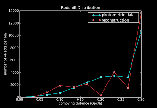
I ran the SDSS CAS data though our working pipeline. I've run on a small data set as a first go -- the same size as what I was running on for the reconstructions with the mock data -- 20,000 points in both the photometric and spectroscopic data sets. The difference here is that both data sets are coming from the same super-set of data (I am randomly picking points from a larger set of Stripe-82 data), so the redshift distributions of the two sets are the same (see below plot). This, in theory, should make the reconstruction easier to do.

Redshift Distributions of photometric and spectroscopic data sets

The Bad News

The correlation functions look really noisy. This is hopefully due to the fact that I am running with 20,000 points instead of 1,000,000 points (before) so hopefully the noise will clear up when I re-run with a larger data set. I wouldn't expect the correlations to look as smooth on a smaller data set as it does with the mock data, because the mock data, by design, traces dark matter populations explicitly, so the dark matter signal is put in by hand. There is also more noise on this data than on the mock data. It is logical to me that we might need higher statistics to get the same strength of signal as we did in the mock data.

The Good News

Even with the noisy correlation functions, the reconstruction looks not too bad. There seems to be a problem at the edges (it seems to be forcing the reconstruction to be zero at redshift zero and thus changing the shape on the low end), but overall it looks pretty good. (At least much better than it's ever looked before). Thoughts Alexia?

I've chosen the binning which looks the best. Like what happened in the mock data the reconstruction changes a lot depending on the binning. However, it looks like I might actually have something working here! Woo hoo!

Next steps

Higher Statistics: I'm not sure if I should run on Eyal's LRGs or on a bigger set of CAS data. The CAS data is easier to do right away, so I might as well set that going (it will take a couple days), and in the mean time I can work on getting my code to read in Eyal's randoms instead of generating it's own. Will talk to Schlegel about this and see what he thinks.

Other Catalogs: According to Eric Huff, Reiko Nakajima has a SDSS catalog with her own calculated photo-z's that she uses for lensing. I will talk to her about this. I also should get in touch with Antonio Vazquez about catalogs.

Optimization: There is quite a few things I can do to make this code run faster. I need to spend some time writing scripts to simultaneously calculate all the correlation functions (right now they are calculated in succession). This should speed up the code by a factor of ten. I also should write scripts so that I can just set a run going and then log-out of the terminal window.

Organizational Note

For a while now I've been creating a log file for each day with the code I use to generate the plots for the blog post that day. I've been keeping these log files locally on my computer, but decided it might be useful for collaborators to have copies of them, and also for there to be a back-up should something happen to my laptop. I've now added these logs to the repository under: repositoryDir/Jessica/pythonJess/logs. The name of the log file is the date of the blog post which the code corresponds to.

Changing Bins

After struggling with a segmentation fault problem, I have run the reconstruction with different bins. The 3D correlation functions seem to be having some problems at small separations (see plot below), need to look into this. The reconstruction still looks ok, although it seems to be very dependent on how many phi bins I use to reconstruct (see Playing with Reconstruction post). I need to get to the bottom of this. Next step, seeing what it looks like on the CAS data.

My Fault

I wanted to play with the binning of my correlation functions, and so tried to run again with different bin sizes. I got the following message when I tried to run the 2D cross correlation:

In [111]: runcrossCorr(argumentFile, corr2dfile, spec2dfile, photo2dfile, nrbins, minRaS, maxRaS, minDecS, maxDecS, minRaP, maxRaP, minDecP, maxDecP, mincorr, maxcorr, corrBins)

sh: line 1: 15436 Segmentation fault ./2dcorrFinal wpsInputs0 >./wps0.dat

sh: line 1: 15445 Segmentation fault ./2dcorrFinal wpsInputs1 >./wps1.dat

sh: line 1: 15447 Segmentation fault ./2dcorrFinal wpsInputs2 >./wps2.dat

sh: line 1: 15449 Segmentation fault ./2dcorrFinal wpsInputs3 >./wps3.dat

sh: line 1: 15455 Segmentation fault ./2dcorrFinal wpsInputs4 >./wps4.dat

sh: line 1: 15460 Segmentation fault ./2dcorrFinal wpsInputs5 >./wps5.dat

sh: line 1: 15462 Segmentation fault ./2dcorrFinal wpsInputs6 >./wps6.dat

sh: line 1: 15471 Segmentation fault ./2dcorrFinal wpsInputs7 >./wps7.dat

sh: line 1: 15473 Segmentation fault ./2dcorrFinal wpsInputs8 >./wps8.dat

sh: line 1: 15482 Segmentation fault ./2dcorrFinal wpsInputs9 >./wps9.dat

sh: line 1: 15484 Segmentation fault ./2dcorrFinal wpsInputs10 >./wps10.dat

sh: line 1: 15489 Segmentation fault ./2dcorrFinal wpsInputs11 >./wps11.dat

sh: line 1: 15495 Segmentation fault ./2dcorrFinal wpsInputs12 >./wps12.dat

sh: line 1: 15508 Segmentation fault ./2dcorrFinal wpsInputs13 >./wps13.dat

sh: line 1: 15548 Segmentation fault ./2dcorrFinal wpsInputs14 >./wps14.dat

sh: line 1: 15596 Segmentation fault ./2dcorrFinal wpsInputs15 >./wps15.dat

Have I mentioned how much I hate Segmentation Faults?

After an hour of debugging I finally figured out that I had left out a line of code that converted from radians to degrees. I really need to put better error checks into the code so that it prints a message when something like this happens, rather than dying.

Kinda mad at the world now.

Time to Get Real

Now that I have a working reconstruction pipeline it is time to run on real SDSS data. I am going to re-run on the data set I have (from CAS database), but I don't believe that the photo-z's are accurate enough to use as the redshifts. To simply use all the spectroscopic data from Sloan isn't going to work because the mask is going to be horribly complicated and I really just want something simple like Stripe 82.

Eyal Kazin has a large catalog of Luminous Red Galaxies that he used to compute the BAO signal. He also has randoms (presumably using a mask) that I could use for calculating the correlation functions. I downloaded this catalog and it only has 105,831 objects in it (3190 in Stripe 82), however the redshift distribution is pretty distinct:

I might be worth trying to reconstruction using his randoms to see what I get. It is probably only 1/2 a day's work to re-write the correlation function to use his randoms instead of generating my own. His random catalog has 15X as many points and has the same redshift distribution (above) and ra, and dec distribution as the data:

The data (blue) falls right on top of the randoms (red)

I have also contacted Eric and Demitri as they have both mentioned having catalog/databases that I might be able to use. I should also contact Antonio.

Python Tip of the Day: I sometimes find that I lose my plotting window. You can close it in the python terminal by the following command: close() and then re-plot to find it again.

Playing with Reconstruction

First selection function:
sf=selection(0.2,0.1,0.05,0.2,bins)


First phi:
Best Reconstruction:
Other reconstructions (not so good):

New selection function:
sf=gals.selection(0,0.05,0.3,10,bins)

New phi:
Best reconstruction:
Other reconstructions:

Success!

I finally got Alexia's new crl working. As far as I can tell the only difference is that getximat expects the errors in xi as an input. For now I am just inputting an identity matrix, as I will need to get the errors by bootstrapping and haven't done that yet.

The function getximat wants a matrix that is the same size as the length of the xiss matrix:
xierr = N.identity(xispec.shape[1],float)

I am reconstructing from 0 to 0.5 Gpc/h using 20 bins. I am renormalizing the reconstructed redshift distribution by the following:
sum(photometric data)/sum(reconstructed data)
This gives the same "number" of objects in both sets.

This is the first reasonable reconstruction I have ever generated. This makes me very very happy. I'm going to play with different binning and selection functions next, but I would like to have at least one blog entry which has a happy ending.

Struggling with Eclipse

I use Eclipse to interface with the SVN repository where Alexia and I share our code. At some point in the last month the repository location at Princeton was moved, and this caused Eclipse to be unhappy. I should be able to change the location of the repository in the following way:

Go to "SVN Repositories" perspective, right click on current repository and "relocate" to new location.

This failed.

So, I had to re-download it manually, transfer files that were newer on my system to the new repository and then update manually, then add the new repository to Eclipse and delete the old one. Annoying!

However, I did discover that there is a way to ignore certain types of files from being checked in using Eclipse. You do this by going to "Pydev Package Explorer" and then right-clicking on a file, and then select "Team" and then "Add to SVN Ignore." This is helpful to not automatically load the large .dat files to the repository.

Now that I have everything working again, time to explore the new crl.py file....

Back to Work (back to Reconstruction)

I need to do a better job of balancing working on both the Newman Project and BOSS Likelihood target selection. I feel like it's been months since I have worked on the Newman stuff. Luckily Alexia was in Mexico and helped me get up to speed again.

Martin White gave me a halo mock catalog (I was using the wrong one for a while) and I have applied the following selection function to the photometric data set:

This corresponds to the following redshift distribution (phi):

The blue line is a histogram of the redshifts of the mock data, and the green line is the phi we are imposing (by both geometry and the selection function, you can see they match pretty well). I believe the difference in these two is based on actual structure, not an problem with implementing the selection function.

On the spectroscopic data, I imposed no selection function, and so the distribution was based purely on the geometry and structure of the data. Because the geometry is a sphere, we expect more objects at greater redshifts (larger volume at greater r):

I decided to start with a small run with data sets of approximately equal size. The photometric data set has 25,887 objects, and the spectroscopic data set has 25,470 objects. The redshift bins are 50 Mpc/h wide and go from 0 - 500 Mpc/h. Here are the 2D cross-correlation functions and the 3D auto-correlation functions of the mock data:

Here is the reconstruction. It is using an old version of crl (I'm having trouble downloading the newest version from the repository). It doesn't seem to be doing that good of a job reconstructing:

Maybe updating crl will help things? Thoughts Alexia?

Notes from the Beach

I have spent the last two weeks at two conferences. First the American Astronomical Society (AAS) 215th Meeting in Washington DC, second Essential Cosmology for the Next Generation: Cosmology on the Beach in Playa del Carmen, Mexico. Both were really helpful for both learning new astrophysics, as well as getting lots of new ideas for my work.

I thought I would summarize here the highlights (with links to talks, and a list of things I would like to look into myself).

Max Tegmark coined the phrase "Goldilocks Galaxies" when talking about the Luminous Red Galaxies (LRGs) in SDSS. This is because "Quasars are too sparse, common galaxies are too dense, but LRGs are just right."

Mark also talked about 21 cm tomography comparing it to the CMB in it's potential importance to cosmology. His description unfortunately was pretty general and I don't think I understand how it works. Need to read a review paper on this. Looks like this might be a good one.

Nicholas Suntzeff had an interesting slide at the end of his talk where he gave advice to young cosmologists about how to be competitive for jobs. I've repeated it below:

• Don’t keep on doing your thesis over and over again
• Establish prominent collaborators and mentors, but appear independent
• Publish, publish, publish. Include useful tables of summary and colorful figures that can be easily captured.
• Apply for external funding
• Luck verus hard work
• Become the leader in your field
• Think carefully about joining large projects with time scales of > 5 years.
• Spergel’s law
• Don’t be afraid to go out on a limb and say something weird (people will remember you).
• The Aaronson effect in obsevations.
• When you apply for jobs, make sure you know all about the department – and brown nose a bit. Write your application as if there is no other job out there. Know your audience.
  

Berian James is a new post-doc at the BCCP starting this spring. He had some ideas about Newman project and had talked to others who are working on similar things (he named John Peacock and Hannah Parkinson at Edinburgh). He also had an interesting idea that it would be great if we could positions from photometry and a redshift distribution and generate a correlation function from these two things. He was wondering if anyone has done this. I should talk to him more about this when he gets to Berkeley.

Dovi Poznanski suggested I look at quasar variability using overlapping Sloan plates. Apparently 20% of the data has multiple epochs. Josh Bloom also told us that we could get good variability information using Palomar data. Nic Ross and I should set up a meeting with him when we get back.

Daniel Matthews is Jeff Newman's graduate student. He presented a poster at the AAS (see Jan 2nd email, subject: poster, he sent me a copy). In this poster he talked about doing redshift distribution reconstructions of "DEEP-like" data. He does something different than what Newman does in his paper. He claimed that he couldn't get Newman's method to work -- this is discouraging. Maybe it's time to try to talk to Newman directly about the project to clarify this?

The Joe Wolf Effect.

Marilena LoVerde discussed lensing of quasars from hydrogen in the ly-alpha forest. I talked to her afterwards and it doesn't seem like this effect his that large, but might be relevant for BOSS/BIG BOSS. The talk isn't posted on the Cosmology on the Beach web page as of right now.

Eyal Kazin has a web page with LRG catalogs. He said he is interested in the Newman Project and is very familiar with SDSS data, and to contact him if we want help. These LRGs might be useful data to use instead of the ones I downloaded from CAS, and don't really trust.

I had some thoughts about if I should request authorship on future DRIFT analysis papers, considering they didn't allow me to publish my work. I don't know what the protocol for this type of thing is, or if it even matters at this point in my career.

I had a great time at these conferences and learned a lot. Time to get back to real work now! Science to follow....

(Award Winning) AAS Poster

Below is my poster from the American Astronomical Society Meeting in Washington DC last week. It is on the likelihood method and initial results.

(Click on image for larger resolution)

I'm currently at the Cosmology on the Beach conference. Sorry for lack of posting. Will post more soon.

Update: This poster won the Best Poster Award at the Cosmology on the Beach conference. Woo hoo!