xmpl_rv, ximat and sximat

Alexia I suggested to look at xmpl_rv (ximat) and sximat to make sure that the interpolation of the xi matrix is in the same location as the xi matrices from the data.

The results are surprising. First of all, the plot of ximat vs sximat is basically a flat line, when plotted log space (click on images to enlarge):

The above plot has sximat, ximat for 3 different binnings (39, 40, and 41) and the plots basically all fall on top of each other. This is from the best "working" reconstruction mock data, described here.

But they don't fall on top of the xi correlation functions from the data:

I thought maybe this was a conversion issue, but I checked and I think they are in the same units. In order to even get the cximat to fall on top of the xi correlation functions you need to divide by 10^4:

Alexia am I doing this right? Is this weird to you?

Different Reconstruction

Here is the reconstruction I ran last night with a different photometric distribution function, below shows the photometric and spectroscopic distributions:

I used the same number of bins and angles as yesterdays post. Here are the correlation functions:

And here are the reconstructions with several different binnings. None of them match as well as yesterdays post, but both 40 and 39 are close-ish:

I talked to Alexia this morning, she suggested that I do the binning sensitivity check and also look at how xmpl_rv (in getximat) compares to sximat. I'm doing that now. Most posts to come shortly.

Here's the code to make the following (also in logs/110509log.py):

import numpy as N

from pylab import *

from matplotlib import *

import crlold as crl

from correlationData import *

import galsphere as gals

import datetime as dt

workingDir = 'run201159_123'

runConstantsFile = './'+workingDir+'/runConstants.dat'

mockLRGfile,photofile,specfile,corr2dfile,corr3dfile,photo2dfile,photoCDfile,spec2dfile,spec3dfile,\

argumentFile,runConstantsFile,wpsMatrixFile,xiMatrixFile,oversample,corrBins,mincorr,maxcorr,boxside,\

xicorrmin,xicorrmax,nxicorr,rbinmin,rbinmax,nrbins,psubsize,ssubsize=readRunConstantsFileAll(runConstantsFile)

rbinspace = int((rbinmax-rbinmin)/(nrbins))

rbins = makeRbins(rbinmin,rbinmax,rbinspace)

#read in masks

minRaP,maxRaP,minDecP,maxDecP,minCDP,maxCDP,minRaS,maxRaS,minDecS,maxDecS,minCDS,maxCDS=readmasks(workingDir)

#Import the photometric redshift distribution

photoCD = readPhotoCDfile(photoCDfile)

#Create a matrix to input the correlation function data

# Write wps Matrix to file

#The number of redshift bins you want to skip for the

#reconstruction (this removes noisy bins from calculation)

skip = 0

makeWPSmatrix2(workingDir,rbins,corrBins, wpsMatrixFile, skip)

#Create a matrix to input the correlation function data

# Write Xi Matrix to file

makeXimatrix2(workingDir,rbins,nxicorr,xiMatrixFile, skip)

#Plot wps correlation functions

numtoplot = int(nrbins-skip) #number of correlation functions you want to display on plot

plotWPS(skip, numtoplot, workingDir, rbins)

numtoplot = 10

plotWPSScreen(skip, numtoplot, workingDir, rbins)

#Plot xi correlation functions

plotXi(skip, numtoplot, workingDir, rbins)

plotXiScreen(skip, numtoplot, workingDir, rbins)

#from commandsAlexia import *

xissfile = xiMatrixFile

wpsfile = wpsMatrixFile

nphibins = size(rbins)

# Read in the data

#spectroscopic autocorrelation function

X=N.loadtxt(xissfile,comments='#')

X=X.T

rs=X[0,:]/1000. #want box units (Gpc, not Mpc)

xispec=X[1:,:] #xi in nspecbins

#2D cross correlation between spec and photo samples

th,rlos,wps=N.loadtxt(wpsfile,comments='#',unpack=True)

th=N.unique(th)

rlos=N.unique(rlos)

#rlos=getcomovingD(rlos) #adjusts from redshift to Mpc/h

rlos=rlos/1000 #want box units (Gpc, not Mpc)

#covariance matrix of wps measurements, wps vector arranged

covar = N.identity(wps.shape[0],float)

xierr = N.identity(xispec.shape[1],float)

# compute the xi matrix using the spec sample,

npbins=39#the number of bins you want reconstructed

reconstructmax = 0.5 #in Gpc

reconstructionmin = 0.0 #in Gpc

phibsize = (reconstructmax - reconstructionmin)/npbins

phibins = linspace(start=reconstructionmin,stop=reconstructmax,num=npbins,endpoint=True)

#phibins =(linspace(2,npbins,num=npbins,endpoint=False)+0.5)*(1./npbins)

sximat=crl.getximat(th,rlos,phibins,rs,xispec,xierr)

# invert to recover phi

phircvd=crl.getCoeff(wps,covar,sximat)

for i in range(len(phircvd.x)):

if (phircvd.x[i] < 0):

phircvd.x[i]=0

print 'the recovered selection function is not normalized.'

outphi4 = phircvd.x

phibins4 = phibins

start = 1

end = npbins - 1

#junkbins = linspace(start=0,stop=0.5,num=100,endpoint=True)

junkbins = phibins

junk = histogram(photoCD/1000., bins=junkbins)

junkdata = junk[0]

plot(junkbins[start:end], junkdata[start:end], 'r.-', label = 'photometric data')

plot((phibins4[start:end]+1.0*phibsize), outphi4[start:end]*sum(junkdata[start:end])/sum(outphi4[start:end]), 'g-', label='reconstruction %i'%npbins)

xlabel('comoving distance (Gpc/h)')

ylabel('number of objects per bin')

title('Redshift Distribution')

from pylab import *

legend(loc=2)

Going back to Working Reconstruction

I spent today trying to reproduce the result from this post when the reconstruction was working on the Mock Data.

I got it working... here is the code (also in ../logs/110509log.py):

#~~~~~~~~~~~~~~~~~

import numpy as N

from pylab import *

from matplotlib import *

import crlold as crl

from correlationData import *

import galsphere as gals

import datetime as dt

workingDir = 'run2010211_1354'

# Create file names

mockLRGfile,photofile,specfile,corr2dfile,corr3dfile,photo2dfile,photoCDfile,spec2dfile,\

spec3dfile,argumentFile,runConstantsFile,wpsMatrixFile,xiMatrixFile=makeFileNames(workingDir)

oversample = 5.

corrBins = 40.0 #should be one more than you want it to be

mincorr = 0.01

maxcorr = 20.0

convo = 180./pi

corrspace = (maxcorr - mincorr)/corrBins

corrarray = makecorrarray(mincorr, maxcorr, corrspace)

nbins = 40

boxside = 1000.0 #in Mpc/h

xicorrmin = 0.001

xicorrmax = 20.0

nxicorr = 40

#make redshift bins

#boxside = 1000.0 #in Mpc/h

rbinmin = 0 #in Mpc/h

rbinspace = boxside/40 #in Mpc/h

rbinmax = boxside/2.0 + 0.0001 #in Mpc/h

rbins = makeRbins(rbinmin,rbinmax,rbinspace)

nrbins = rbins.size - 1

photoCD = readPhotoCDfile(photoCDfile)

#Create a matrix to input the correlation function data

# Write wps Matrix to file

#The number of redshift bins you want to skip for the

#reconstruction (this removes noisy bins from calculation)

skip = 0

makeWPSmatrix2(workingDir,rbins,corrBins, wpsMatrixFile, skip)

#Create a matrix to input the correlation function data

# Write Xi Matrix to file

makeXimatrix2(workingDir,rbins,nxicorr,xiMatrixFile, skip)

#Plot wps correlation functions

numtoplot = int(nrbins-skip) #number of correlation functions you want to display on plot

numtoplot = 10

plotWPSScreen(skip, numtoplot, workingDir, rbins)

pylab.legend(loc=1)

#Plot xi correlation functions

plotXiScreen(skip, numtoplot, workingDir, rbins)

# compute the xi matrix using the spec sample,

npbins=40#the number of bins you want reconstructed

reconstructmax = 0.5 #in Gpc

reconstructionmin = 0.0 #in Gpc

phibins = linspace(start=reconstructionmin,stop=reconstructmax,num=npbins,endpoint=True)

#phibins =(linspace(2,npbins,num=npbins,endpoint=False)+0.5)*(1./npbins)

sximat=crl.getximat(th,rlos,phibins,rs,xispec,xierr)

# invert to recover phi

phircvd=crl.getCoeff(wps,covar,sximat)

for i in range(len(phircvd.x)):

if (phircvd.x[i] < 0):

phircvd.x[i]=0

print 'the recovered selection function is not normalized.'

outphi4 = phircvd.x

phibins4 = phibins

start = 1

end = npbins - 1

#junkbins = linspace(start=0,stop=0.5,num=100,endpoint=True)

junkbins = phibins

junk = histogram(photoCD/1000., bins=junkbins)

junkdata = junk[0]

plot(junkbins[start:end], junkdata[start:end], 'r.-', label = 'photometric data')

plot((phibins4[start:end]+1.0*phibsize), outphi4[start:end]*sum(junkdata[start:end])/sum(outphi4[start:end]), 'g-', label = 'phi')

plot(phibins4[start:end],outphi4[start:end]*sum(junkdata[start:end])/sum(outphi4[start:end]),'c.-',label='reconstruction %i'%npbins)

#plot((phibins4[2:]-1.5*phibsize)/1000, phi[2:]*size(photoCD), 'g-', label = 'phi')

xlabel('comoving distance (Gpc/h)')

ylabel('number of objects per bin')

title('Redshift Distribution')

from pylab import *

legend(loc=2)

#~~~~~~~~~~~~~~~~~

It involved reverting back to an old version of crl (I saved it as crlold.py) and an older version of the plotting.

Here are the correlation functions:

I am getting the same problems with slight changes to the binning, changing how well the reconstruction works. For instance the best reconstruction is here (with 40 bins):

But if I change to 39 or 41 bins, I get a very different reconstruction:

Which makes me wonder if was just dumb luck that it worked for that particular binning in the first place.

I'm also running with a more interesting photometric distribution function to see how that looks. More to come....

Computing Time

One interesting thing I've realized in trying to compare the 2D auto-correlation with the 3D auto-correlation (on the same files) is that the 2D auto-correlation takes MUCH longer to compute than the 3D. This is strange because in this test they are computing the same number of pairs, well barring some differences in the gridding. I must be doing something very inefficient with the 2D calculation, or measuring pairs out to much larger distances than in the 3D case. The 3D auto-correlation function took less than a minute to compute, and the 2D auto-correlation function is still running, and it's been 51 minutes.

Here are the 2D and 3D autocorrelation functions on the whole set (on big redshift bin)

Below is the 3D and 2D autocorrelation on a smaller (100Mpc/h) redshift bin:

At redshift (well actually comoving distance 350 Mpc/h), what are these angular separations in Mpc/h?

What noise levels would be expect just from shot noise?

How do we expect the slopes to compare?

I talked to David, Eric, Nic and Matt about this. They gave me some references to check out and also suggested that (just as a check) I set the redshifts of the 3d correlation function to all be the same, and then calculate the 3D and 2D, and compare them, they should basically be the same then, or at least proportional to each other.

David also suggested (as a way to figure out where my troubles are coming from.... to go back to the mocks, when the reconstruction was working)... and to then try applying the BOSS Geometry to these mocks and see if I can get the code to work on the mocks with the BOSS Masks. Then once that is working, swap in the BOSS data.

It's worth a try!

References to read:

Dodelson

Peebles 1980

Limber 1954

Still need to do the binning experiments that Alexia suggested. So much to do, so few hours in the day.

BOSS Reconstruction Plots

Here is a reconstruction I tried on the BOSS data. I was hoping that fixing the 2D correlation function might help things, but it doesn't seem to be working that well. Here are the correlation functions:

The 2D correlation functions are still nosier, which is mystifying because they have more objects that are being correlated. I can only assume this has something to do with the different clustering properties of the two sets. I am going to try doing the 2D correlation function on the same files as the 2D and to see if it is still as noisy. If it is, then perhaps this signifies there is still a problem there.

The reconstructions aren't great, but they aren't bouncing around as much as they were before either.

Masked BOSS and SDSS Data

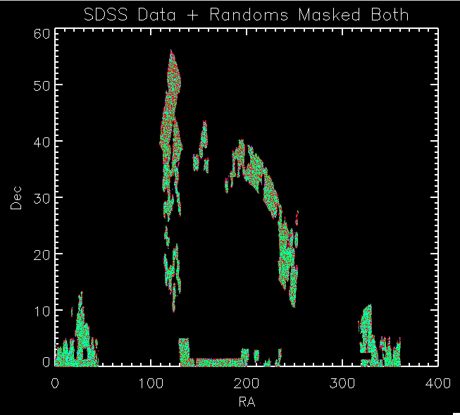
Here are my photometric and spectroscopic data sets, masked so that they have the same footprint in the sky:

Whole Footprint (photometric)

Red = Data, Green = Randoms

Up-close patch (photometric)

Red = Data, Green = Randoms

Whole Footprint (spectroscopic)

Magenta = Data, Cyan = Randoms

Up-close patch (spectroscopic)

Magenta = Data, Cyan = Randoms

Whole Footprint (both)

Spectroscopic: Magenta = Data, Cyan = Randoms

Photometric: Red = Data, Green = Randoms

Up-close patch (both)

Spectroscopic: Magenta = Data, Cyan = Randoms

Photometric: Red = Data, Green = Randoms

Distribution of Dec (spectroscopic)

Magenta = Data, Cyan = Randoms

Distribution of Dec (photometric)

Red= Data, Green = Randoms

Distribution of Dec (both)

Spectroscopic: Magenta = Data, Cyan = Randoms

Photometric: Red = Data, Green = Randoms

Distribution of RA (spectroscopic)

Magenta = Data, Cyan = Random

Distribution of Dec (photometric)

Red= Data, Green = Randoms

Distribution of RA (both)

Spectroscopic: Magenta = Data, Cyan = Randoms

Photometric: Red = Data, Green = Randoms

Distribution of Redshift (z) (spectroscopic)

Magenta = Data, Cyan = Randoms

Distribution of Redshift (z)

Red = spectroscopic redshifts, Magenta = photometric photo-z's

Matching Angular Correlation Function

After banging my head against my code for a while, I seem to finally have a 2d correlation function result that matches the literature....

Published result (from Ross 2007):

Mine:

The values match!

This is an autocorrelation. I want to make sure it doesn't change significantly when I do a cross correlation, then I am going to try and see how it looks when I run in on several bins.

Min